We create custom-built backtesting software in languages like C++ and python for individual traders and institutions to test and optimize their strategies. We also offer general algorithmic trading consulting services.
Finding that backtesting doesn’t seem to work for you? This article may help you understand the statistical reasons for this.
We create backtesting software for all asset classes including backtesting strategies on equities, FX, options, futures and cryptocurrencies.
Whether you’re a lone day trader looking to test your strategy, or a sizable organisation looking for get your feet wet with algorithmic trading and machine learning, our cloud-based quant consulting service has got you covered. This includes:
Python scripts which can evaluate your strategy for different parameters and determine the parameters that give optimal profitability.
Applications which use analyse large amounts of data, use machine learning techniques to find statistically significant signals, and find the optimal way to combine all meaningful signals into a single strategy.
Software to automate your strategies by connecting directly to the exchange to grab the latest price information and post buy/sell orders.
There are many advantages of custom-built backtesting software over the simple built-in functionality offered by some exchanges:
Code offers unfettered ability to do complex calculations on historical data, including analysing for the presence sophisticated technical analysis patterns.
The software can analyse a wide variety of datasets when making trading decisions, including data from other assets and data from outside the exchange.
The power of python – make use of python’s mathematical tools, machine learning and data analysis libraries
The software can grow in scope and complexity as your business grows, as you expand into new strategies and products.
Partner with our experienced PhD quants to supercharge your trading business. Contact us today to discuss how we can design custom-built backtesting software to meet your needs.
To learn more about what’s involved in automating a strategy, see our simple guides for using python to connect to Interactive Brokers and Binance.
Looking for PhD quantitative support and risk management for your cryptocurrency business? Look no further! Contact us to learn how our quants can help.
As decentralized finance continues to grow in size, there is increasingly a need to quants (quantitative analysts) to bring to bear their skills from the world of traditional finance. Due to the relative immaturity of the industry, there is a huge opportunity for cryptocurrency startups to gain a competitive advantage through quantitative skills and tools.
Applications include derivative pricing models, risk modelling including market risk, credit risk and liquidity risk, and developing and backtesting trading algorithms. There are even many novel applications including the mathematics of decentralized oracles and so-called automated market makers.
We offer cloud-based PhD quant consulting and advisory services to the defi industry, all conveniently delivered remotely to anywhere in the world.
Decentralized finance needs a decentralized quant consulting service!
Derivative pricing models
The cryptocurrency derivatives market is still in its early stages. From TradFi, we already have the mathematical techniques to price options in the form of Black-Scholes. And we even have the tools to price exotic derivatives like American, Asian and barrier options. However, we do need sufficient liquidity in the options market in order to derive implied volatilities. We can develop robust libraries of derivative pricing models so your firm can price any kind of cryptocurrency derivative. See our main article on Cryptocurrency Derivatives.
Risk modelling for defi
With the crypto industry continuing to grow in size, risk management should play as important a role in managing customers and assets as it currently does in conventional finance. Given a number of high profile collapses in the industry, effective and reputable risk management could help to allay customer concerns about holding digital assets or interacting with your firm. It’s particularly useful to consider how the extensive existing literature on risk and risk modelling can be carried over to the crypto space. Market risk and liquidity risk modelling are standard challenges arising in other kinds of finance, and one can consult the literature in order to develop similar frameworks for the crypto space. We do however need to take due notice of the higher volatility which creates some additional challenges.
Market risk
There’s some uncertainty about whether digital assets should be modelled more like exchange rates or more like equities. But there’s not doubt that exchange rates between two digital currencies or between a digital currency and a conventional currency exhibit a high degree of volatility, raising some new challenges for market risk modelling
Borrowing and lending businesses have to take collateral to insure their loans. Similarly, exchanges need to take margin to ensure counterparties can meet their obligations when trades move against them. In both cases, firms are exposed to market risk on the value of the collateral, which could also be interpreted as FX risk between the relevant currencies where multiple cryptocurrencies are involved. In particular for borrowing and lending, one needs to be concerned about changes in relative value between collateral in one token and loaned amount in another. A mathematical model is needed which can can set parameters like the LTV (loan to value ratio) or liquidation trigger level in order to avoid the value of the collateral ever falling below the value of the loaned amount.
A standard way to model market risk is VaR (value at risk). We calculate the relative shift in each asset or market variable over each of the last 250 days, and apply each shift to today’s portfolio. We can then calculate the 99% worst quantile (typically assuming normally-distributed price moves) and make sure margin/LTV is sufficient. Actually, it may be advisable to work out what the liquidation window would be, and use that as our timeframe for VaR calculations. This may have implications for how much collateral you’re comfortable holding in any given coin.
Liquidity and execution risk
In addition to market risk, crypto firms are exposed to liquidity risk when trying to dispose of assets and collateral. The larger a firm grows and the larger its market share becomes, the more liquidity risk becomes a key concern. Liquidity risk may be of particular concern for emerging markets such as digital currencies.
Modelling liquidity risk involves looking not just at the mid price of the assets (as market risk tends to), but also considering the market depth and bid-ask spread. Both of these quantities can be examined in a VaR framework in a similar way to market risk. Large spreads are likely correlated to adverse price moves. Some research indicates they may not be normally distributed as is often assumed in market risk. Data analysis can be performed to determine the appropriate spread modelling assumptions for cryptocurrencies.
One can also consider modelling market risk and liquidity risk together in one model, looking at the 99% quantile of adverse price/spread/market depth moves and backtesting a portfolio or risk management protocols against the historical data or hypothetical scenarios.
Of relevance here also are liquidation algorithms / order splitting. While some illiquidity scenarios will be completely outside our control, in other scenarios the crisis arises only if we try to transact too much too quickly (which of course we may have good reason to attempt in a stressed scenario). Thus researching liquidation algorithms and backtesting them are important also.
In particular, it’s important to backtest against a stressed period in the market’s history, to understand how we would respond. This would include situations where collateral value declines dramatically or quickly, many customers wish to withdraw their collateral simultaneously, or periods of higher than usual volatility.
Another important tool is scenario analysis. This is where we consider a range of hypothetical qualitative and non-modellable scenarios, such as liquidity providers shutting down completely, to evaluate how we would respond.
Correlation and principal component analysis (PCA)
Since cryptocurrencies move together to a significant extent, we can separate market risk into systematic risk (i.e. FX rates between cryptocurrencies and USD, which could perhaps be taken as BTCUSD) vs idiosyncratic risk (cryptocurrencies moving independently of each other, ETHBTC for example).
If both the asset and the collateral are digital currencies (and not pegged to a conventional currency), then their price relationship is not affected by an overall move in the crypto space. Thus we would be interested in looking at the risk of relative movement only.
We can start with a correlation analysis of price moves over different time intervals of both traditional and digital currencies. Below shows the correlations of one day price moves over a one year period. It’s clear that there is significant correlation.
We can also do PCA (principal component analysis) to determine how the various coins relevant to the firm move together / contrary to each other. This helps us to understand what benefit is derived from diversification. A PCA analysis is often done on rates curves to determine to what extent short / long tenors move together.
The below PCA analysis shows that 75% of the variance in the price shifts can be explained by all coins moving in the same direction (notice how in the first vector/row all values have the same sign). Interestingly, 9% of the variance can be explained by DOGE moving contrary to all the other coins (notice how it is the only one with a positive value in the second row). The next two rows, explaining 4.7% and 4.5% of the variance respectively, show the coins moving in different directions to each other.
[75%, 9%, 4.7%, 4.5%]
Backtesting and trading algorithms
We design software to backtest, optimize or automate trading or investing strategies.
Backtesting can be performed on historical data, or on hypothetical synthetic data to test the strategy against a wide range of possible market conditions. Usually, trading strategies have a range of possible parameters which we can set for optimal profitability by examining their behaviour on historical data. If you’re still placing your buy and sell orders manually, we can automate execution by writing code to interact directly with the exchange. This not only allows faster reaction, it also allows sophisticated data analysis and machine learning to be incorporated into your strategy. And automation is particularly important for crypto markets which still operate even while you sleep.
The benefits of backtesting actually extends beyond trading. Almost any business or risk strategy can be backtested against historical or hypothetical data in order to test the profitability or robustness of the business.
How does an decentralized oracle convert multiple data sources into a single price or datum? For example, some data sources (for example, different exchanges) may receive different weighting, and more recent data points may be weighted differently than older ones. The oracle might also trim the data between two quantiles to remove the influence of outliers. Some decentralized oracles offer a reward for participants that submit data close to the final price, such as Flare Time Series Oracle (FTSO). How would you go about succeeding as such a participant, or just predicting the final price for your own use? This is where machine learning algorithms come in.
We can build predictive algorithms for decentralized oracles, using machine learning, which predict how oracles combine a large number of inputs into a final output.
Automated Market Makers
Automated market makers, or AMMs, provide liquidity to the market by allowing exchange between two or more cryptocurrencies. They do this by incentivizing people to contribute coins to the pool, and by penalizing the exchange rate if the liquidity ratio swings too far in the direction of one of the coins.
The mathematics around profit and risk of automated market makers and the liquidity tokens they issue require some careful thought. We can conduct this analysis and conduct backtesting of your business strategy.
For details on the Uniswap algorithm, see this article on the CURVE exchange.
The relative immaturity of crypto markets may mean there are more opportunities for arbitrage than on more conventional markets. In this article, we investigate whether price moves in crypto coins are correlated. Specifically, we see whether the last three price moves in a selection of coins can be used to predict the next move in a coin of interest. You could consider this strategy to be a type of statistical arbitrage, or a pairs trading strategy (albeit over a small interval of time).
We implement a vector autoregression model on a select of nine major crypto coins, whose tickers are: SOL-USD, BTC-USD, ETH-USD, BNB-USD, XRP-USD, ADA-USD, MATIC-USD, DOGE-USD, DOT-USD. All data is grabbed directly from Yahoo Finance using the yfinance python package. We use one week of data (the most recent at the time of writing) and a 1 minute time interval.
A VAR model is a variety of linear regression that attempts to predict the next move of a particular coin, based on the last few price moves of the coin and all the other coins. The idea is two-fold. Firstly, if two coins tend to correlate but one moves first, it may portend a move of the other coin. Secondly, the VAR model will attempt to find a trend in the coin itself. In fact, a VAR model includes a moving average crossover as a subset of what it can fit. An interesting feature is that it can potentially use moving averages in other coins as a predictive signal. However, I only used the three previous price moves as inputs to the model as using more than this didn’t appear to improve the result in this case.
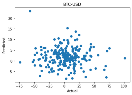
The results show that the algorithm is effective at predicting the next move of many coins, but does not appear to be effective for bitcoin.
Results
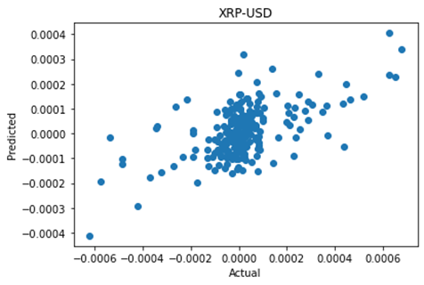
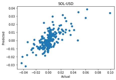
The code produces a scatterplot of the actual vs predicted price moves, along with the correlation and p value between the two. Note that since the code grabs the most recent data at the time of execution, the numbers may differ between runs. Below I show two coins where the algorithm is effective and one where it isn’t.
XRP-USD shows a strong correlation of 0.59 between the actual and predicted next move, with a negligible p value demonstrating statistical significance.
By contrast, BTC-USD shows a poor correlation of 0.015 and a p value of 0.8 showing no statistical significance at all. My interpretation of this is that the smaller coins are more likely to be affected by price moves in Bitcoin, rather than the other way around.
For many coins, the algorithm is able to predict the next price move with strong correlation. Thus, the algorithm could be the starting point for an effective strategy for a variety of cryptocoins.
Future development
A good next step for developing this idea would be to explore using a time interval of less than one minute. Particularly in live prediction, one would not want to wait up to a minute to analyse the data and make a decision. Ideally, the algorithm would analyse and take action every time the exchange updated the price of one or more coins. It would also be interesting to develop a model that accesses data for a very large number of assets (including not just crypto but other asset types, economic parameters etc) and search for correlations. One could eventually explore using big data / machine learning techniques to search for these relationships.
Python code
Below is the python code used for this article. You can specify which coin you are trying to predict using the index_to_predict variable. In order to protect against overfitting to a particular piece of historical data, the variable test_fraction specifies how much of the data to set aside for testing (I’ve used the last 20%).
import numpy as np
import pandas as pd
import matplotlib.pyplot as plt
from statsmodels.tsa.api import VAR
from statsmodels.tsa.statespace.tools import diff
from scipy.stats import linregress
import yfinance as yf

# Set data and period interval
period = "1w"
# Valid intervals: [1m, 2m, 5m, 15m, 30m, 60m, 90m, 1h, 1d, 5d, 1wk, 1mo, 3mo]
interval = '1m'

# Number of previous moves to use for fitting
VAR_order = 3

tickers = ["SOL-USD","BTC-USD","ETH-USD","BNB-USD","XRP-USD","ADA-USD","MATIC-USD","DOGE-USD","DOT-USD"]
# Specify which coin to forecast
index_to_predict = 0
test_fraction = 0.2 # fraction of data to use for testing

data = yf.download(tickers = tickers,  # list of tickers
                period = period,         # time period
                interval = interval,       # trading interval
                ignore_tz = True,      # ignore timezone when aligning data from different exchanges?
                prepost = False)       # download pre/post market hours data?

X = np.zeros((data.shape[0],len(tickers)))

for (i,asset) in enumerate(tickers):
    X[:,i] = list(data['Close'][asset])

# Deal with missing data.
NANs = np.argwhere(np.isnan(X))
for i in range(len(NANs)):
    row = NANs[i][0]
    X[row,:] = X[row-1,:]

# Difference data
Xd = diff(X)

# Determine test and fitting ranges
test_start = round(len(Xd)*(1-test_fraction))
Xd_fit = Xd[:test_start]
Xd_test = Xd[test_start:]

model = VAR(Xd_fit)
results = model.fit(VAR_order)
summary = results.summary()
print(summary)

lag = results.k_ar

predicted = []
actual = []
for i in range(lag,len(Xd_test)):
    actual.append(Xd_test[i,index_to_predict ])
    predicted.append(results.forecast(Xd_test[i-lag:i], 1)[0][index_to_predict])

plt.title(tickers[index_to_predict])
plt.scatter(actual, predicted)
plt.xlabel("Actual")
plt.ylabel("Predicted")

print(linregress(actual, predicted))
In a couple of previous articles, we backtested and optimized a moving average crossover strategy for both Bitcoin and FX.
Now while backtesting on historical data is a key part of developing a trading strategy, it also has some limitations that are important to be aware of.
Firstly you have the issue that you usually have a limited amount of historical data. And even if you could obtain data going back as many years as you wanted, the relevance of older data is questionable. Also, when you have a finite amount of data, there’s always the problem of overfitting. This occurs when we optimize too much for the idiosyncrasies of one particular dataset, rather than trends and characteristics which are likely to be persistant.
And even if you had say, ten years of data, if there happened to be no GFC during those ten years you’d have no idea how the strategy would perform under that scenario. And what about scenarios that have never happened yet? A strategy that is perfectly optimized for historical data may not perform well in the future because there’s no guarantee that future asset and market behaviour will mimic past behaviour.
This is where backtesting using synthetic data comes in.
Synthetic data is data that is artificially generated. It can be generated so as to try to mimic certain properties of a real historical dataset, or it can be generated to test your strategy against hypothetical scenarios and asset behaviour not seen in the historical data.
Now the downside of backtesting using synthetic data is that it may not accurately depict the real behaviour of the asset. However, even real historical data may not be representative of future behaviour.
With synthetic data, one can generate any amount of data, say 100 years or even more. This means:
No problems with overfitting – you can generate an unlimited amount of data to test whether optimized parameters work in general or only on a specific piece of data.
The large amount of data should contain a wider range of possible data patterns to test your strategy on.
Mathematical optimization algorithms for finding optimal parameters work perfectly as they can work with smooth, noise free functions.
It’s easy to explore how properties of the data (eg, volatility) affect the optimal parameters. This can ultimately allow you to use adaptive parameters for your strategy, which change based on changing characteristics of the data such as volatility.
It allows you to test how robust your strategy is on hypothetical scenarios that might not have occurred in the historical data. For example, if you backtested your strategy on data with lower volatility, will it still be profitable if the asset volatility increases? Would your strategy be profitable (or at least minimize losses) during a market crash?
How to generate synthetic data
In general, when generating asset paths for stocks, cryptocurrencies or exchange rates, the starting point is geometric Brownian motion. For some applications you may wish to add random jumps to the Brownian motion, the timing of which can be generated from a Poisson process.
However, when generating synthetic data for backtesting purposes you will probably find that your strategy is completely ineffective when applied to geometric Brownian motion alone. This is because real asset price data contains non-random features such as trends, mean reversions, and other patterns which are exactly what algorithmic traders are looking for.
This means that we have add trend effects to our synthetic data. However, it does raise a significant issue: how do we know that the artificial trends and patterns we add to the data are representative of those present in real data?
What you’ll find is that the profitability of the strategy is largely determined by the relative magnitudes of the geometric motion and the trend term. If the trend is too strong, the strategy will be phenomenally profitable. Too weak, and the strategy will have nothing but random noise to work with.
We will not concern ourselves too much with generating highly natural or realistic data in the present article as our primary purpose here is to study how synthetic data can allow us to explore the behaviour of the strategy, and how its optimal parameters relate to the properties of the data.
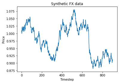
We generate synthetic FX data using the code below. We assume the initial FX rate is S0 = 1, and volatility is 10%. Since, barring some kind of hyperinflation event, an exchange rate does not usually become unboundedly large or small, we add in some mean reversion that tends to bring it back to its original value.
While there are many ways of defining a trend, our trend is a value which starts at 0 and drifts randomly up or down due to it’s own geometric brownian motion. There is also a mean reversion term which tends to bring the trend back to 0. The trend value is added to the stock jump each time step.
To get an idea of what our synthetic data looks like, below I’ve generated and plotted 1000 days of synthetic FX data.
Backtesting an FX moving average strategy on synthetic data
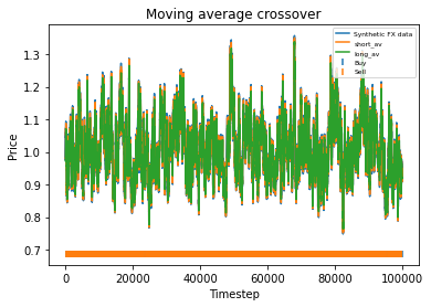
We generate 100,000 days of synthetic FX data and run our moving average backtesting script from the previous two articles.
Plotting 100,000 datapoints on a graph along with the short and long moving averages produces a seriously congested graph. However, we can see that the synthetic data does not stray too far from its initial value of 1. In fact, we could probably stand to relax the mean reversion a bit if it was realistic data we were after. The greatest variation from the initial value of 1 seems to be about 30% which is too low over such a long time period. Now the profitability of the strategy is not particularly meaningful here, since as mentioned it is largely determined the strength of the trend as compared to the Brownian motion that the user specifies. If the strategy is profitable, the profit will also be very high when the strategy is executed over 100,000 days.
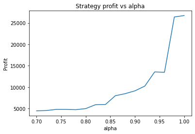
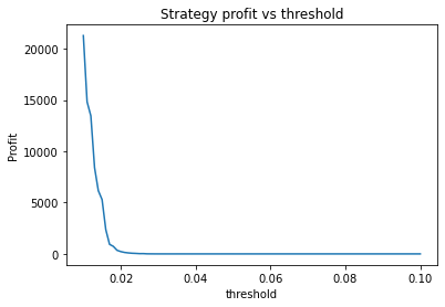
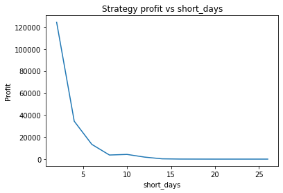
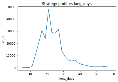
What is interesting though, is to strengthen the trend of the data (say, changing 0.7*trend to 1*trend in the earlier code snippet) and plotting graphs of profitability vs parameter values. When backtesting against real historical data, we often found that the resulting graphs were noisy and multi-peaked, making it difficult to determine the optimal parameters. Using a much larger quantity of synthetic data with a strong trend, we find the graphs are clean and clear.
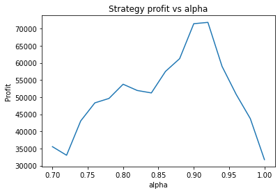
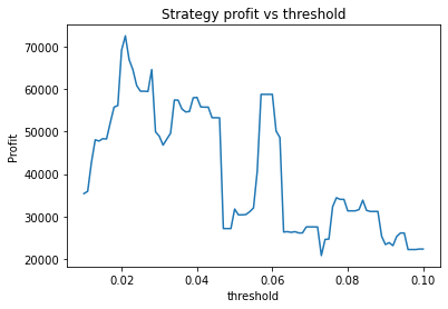
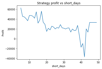
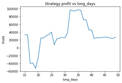
We can clearly see that the optimal values are alpha close to 1, say 0.975, threshold as small as possible, short days also very small and long days about 22.
What happens if we make the volatility of the data smaller by a factor of 3?
It seems the optimal alpha has reduced to about 0.9. Also, the optimal number of days used for the long term average has increased from low twenties to high twenties.
It’s unlikely you’d be able to extract this insight from backtesting on historical data. Firstly, you wouldn’t be able to adjust the volatility of the data on a whim, and the graphs would be too noisy to clearly see the relationship. What this example illustrates is that synthetic data can be used to study how various properties of the data affect the optimal parameters of the strategy. This could be used to create a strategy with “adaptive” parameters which change based on the most recent characteristics of the data, such as volatility. A very simple example of this would be increasing the number of days used in the long term average during periods of high volatility.
Testing stressed artificial scenarios
Another utility of synthetic data is the ability to generate particular scenarios on which to test your strategy. This might include periods of high volatility, steeply declining or rising data, or sudden jumps. To achieve this, one can generate some synthetic data using the method already described, and then manually adjust the data points to create a particular scenario. This will help you to understand what kind of data may “break” your strategy and how you might be able to adjust parameters, or add in additional conditional behaviour or fail safes.
Some distinguishing characteristics of Forex trading, as opposed to stock trading, is 24 hour trading, virtually no limit on liquidity, and the potential for significant leverage on trades. These features are all fortuitous for an algorithmic approach to trading.
The crossing over of short and long term moving averages is a well-known signal used in algo trading. The idea is that when the short term average rises above the long term average, it could indicate the price is beginning to rise. Similarly, when the short term average falls below the long term average, it could indicate the price is beginning to fall.
In a previous article, we investigated backtesting a moving average crossover strategy on bitcoin. We found that our backtesting allowed us to pick optimal parameters for the strategy that very significantly improved its profitability, and resulted in a far higher return than simply buying and holding the asset.
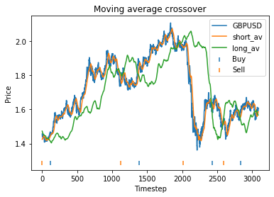
In this article we conduct the same analysis on four currency pairs – GBPUSD, EURUSD, AURUSD and XAUUSD. Forex data going back to January 2001 has been sourced from forextester.
We assume that the trader initially converts one USD to the other currency, converts back and forth between the two currencies based on whether he believes the exchange rate is trending up or down, and converts back to USD at the end. The profit is compared against that of simply holding the non-USD currency for the entire time.
As before our strategy has four parameters to optimize: alpha, threshold, short days and long days.
short_days – The number of days used for the short term average
long_days – The number of days used for the long term average
alpha – This is a parameter used in the exponential moving average calculation which determines how much less weight is given to data further in the past. A value of 1 means all data gets the same weighting.
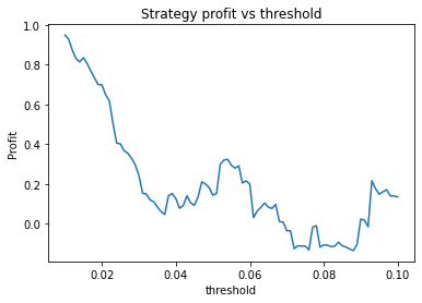
threshold – A threshold of 10% means that instead of executing when the two averages cross, we require that the short average pass the long average by 10%. The idea is to prevent repeatedly entering/exiting a trade if the price is jumping about near the crossover point.
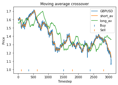
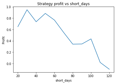
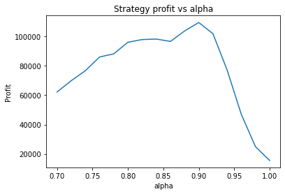
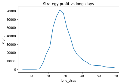
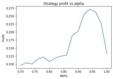
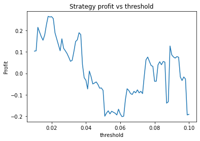
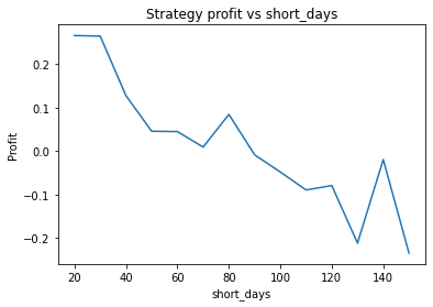
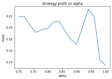
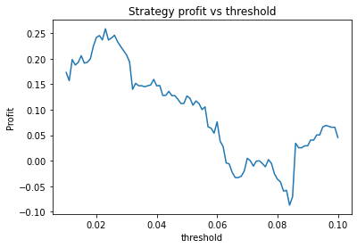
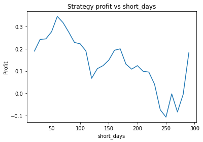
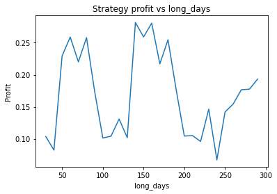
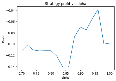
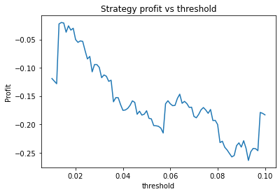
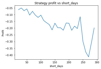
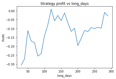
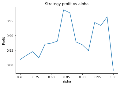
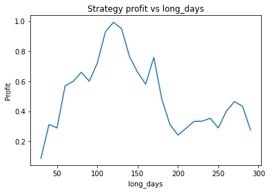
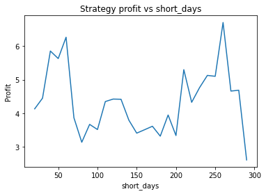
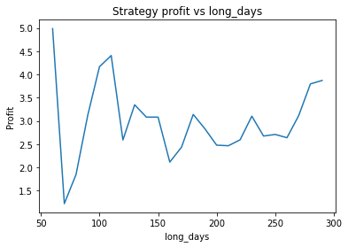
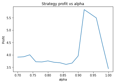
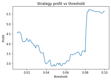
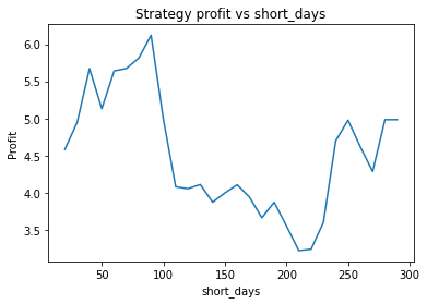
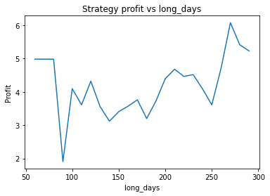
We plot graphs showing the profit of the strategy for different values of each parameter. From these graphs, we choose optimal parameters for each currency pair. The full results, graphs and the python code used in this analysis are available below.
Conclusions
There are many pitfalls and caveats when doing this kind of optimization, and what seem like the optimal parameters should never be accepted naively. Things to keep in mind:
We are finding the optimal parameters on a particular piece of historical data. There is no guarantee that these parameters will be effective on future data which may differ in significant ways from historical data.
We have to be careful we are not “overfitting”, which occurs when we optimize too much for the idiosyncrasies of our particular dataset, rather than trends which are likely to persist. One way to guard against this is to split the data into pieces and perform the optimization on each piece. This gives an idea of how much variation to expect in the optimal parameters.
A question that arises in our set of graphs below, is how to choose parameters when the graph of profit against parameter value is noisy, multi-peaked or has highly unstable peaks (eg two close together parameters values that have radically different profitability).
We find different currency pairs exhibit differing optimal parameters. However, a critical question is how much of this variation is genuine, and can be expected to hold into the future, and how much is just noise in the data. However, generally speaking we find the following parameters are effective in most cases:
Alpha large, say 0.95
Threshold small – 0.01 or 0.02. This indicates that the threshold variable is often not useful and could perhaps be removed.
Short days between 30 and 60
Long days between 120 and 160
This information is certainly useful, and helps us to configure our moving average strategy much better than if we were merely guessing at, for example, how many days to take the long average over. It’s important to realise that even the most carefully optimized strategy can fail when conditions emerge that were not present in its historical backtesting dataset.
It’s worth noting that these optimal parameters differ from those we found for bitcoin. In that case, we found a long days parameter of just 35 and a short days parameter of just 10 were optimal. This probably reflects the much higher volatility of bitcoin as compared to Forex markets.
This article highlights some of the difficulties involved in backtesting strategies on historical data. One way to resolve many of these issues is to test and optimize your strategy on synthetic data. This will be the subject of a future article.
Results
GBPUSD
Strategy profit is: 0.2644639031872955
Buy and hold profit is: -0.23343631994507374
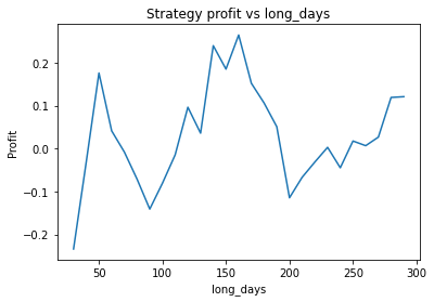
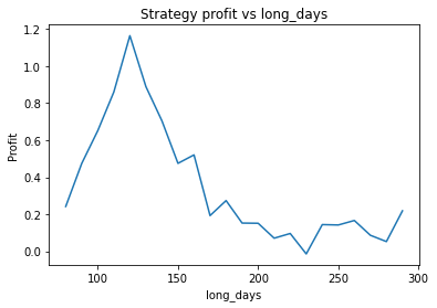
We find that the optimal alpha is about 0.95. The threshold graph displays a general downward trend so we choose threshold = 0.02. The short days graph displays a clear downward trend so we choose short_days = 30. The long days graph displays a peak at about 160. It’s not entirely clear whether or not this peak is simply an artifact of the particular dataset we are looking at. If we believed this, we might choose a value more like 300 since the graph displays a general upward trend. Regardless, we choose long_days = 160 in this case.
Using these values, our strategy has a profit of 0.26 USD, vs a loss of 0.23 USD from buying and holding GBP.
Another thing we can do here is guard against overfitting by splitting the dataset into two halves, repeat the process on each piece, and seeing whether the optimal parameters change much. Surprisingly, we find that the optimal parameters are about the same for both halves of the data. This will often not be the case, however.
First half:
Second half:
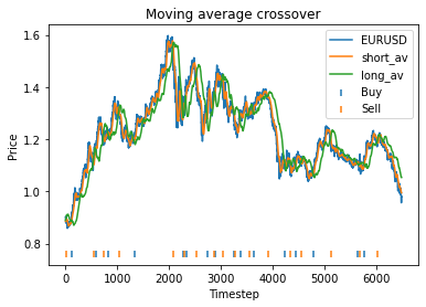
EURUSD
Strategy profit is: 0.9485592864080428
Buy and hold profit is: 0.086715457972943
Using these values, our strategy has a profit of 0.95 USD, vs a profit of 0.087 USD from buying and holding EUR.
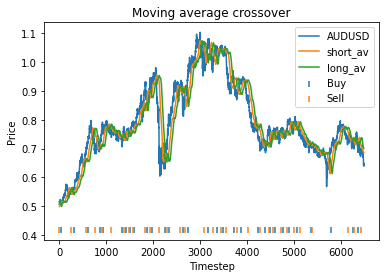
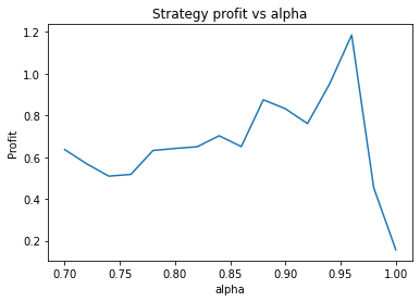
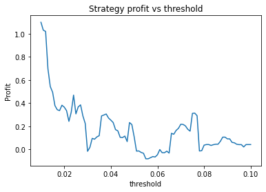
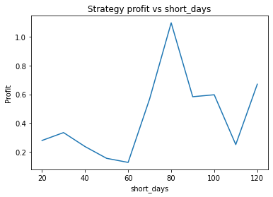
AUDUSD
Strategy profit is: 1.0978809301386634
Buy and hold profit is: 0.24194800155219265
From these graphs, it seems an optimal choice of parameters might be apha = 0.95, threshold = 0.01, short_days = 80, long_days = 125. Using these parameters are strategy returns 1.1 USD vs 0.24 USD for buy and hold. However, it’s also clear that the parameters alpha, short_days and long_days are highly unstable. The optimum occurs at a narrow peak, with relatively nearby parameter values giving dramatically lower performance.
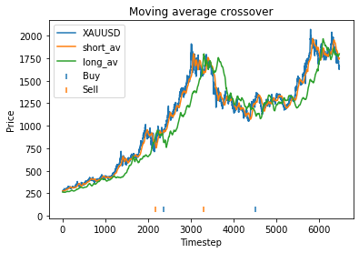
XAUUSD
Strategy profit is: 6.267892218264149
Buy and hold profit is: 4.984864864864865
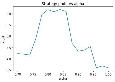
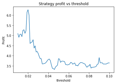
We first try parameters of alpha = 0.85, threshold = 0.02, short_days = 60, long_days = 300. This results in a profit of 6.27 USD versus a buy and hold profit of 4.98 USD.
Interestingly, there is another optimum given by alpha = 0.95, threshold = 0.1, short_days = 60, long_days = 300.
Strategy profit is: 5.640074352374969
Buy and hold profit is: 4.984864864864865
The way the threshold and alpha graphs change when we change the base threshold and alpha shows the interdependence of the parameters.
Python code
The python code used in this analysis is made available below.
import numpy as np
import pandas as pd
import matplotlib.pyplot as plt
from scipy.optimize import minimize
#data = pd.read_csv("GBPUSD.txt")
idx = 0
Names = ["GBPUSD", "EURUSD", "AUDUSD", "XAUUSD"]
Name = Names[idx]
data = pd.read_csv(Name + ".txt")
#data = data.iloc[::-1] #reverses order of dates
# Filter for daily data only
data = data.drop_duplicates(subset=['<DTYYYYMMDD>'], keep='last')
close = np.array(data["<CLOSE>"])
#close = close[:3389]
def moving_avg(close, index, days, alpha):
# float values allowed for days for use with optimization routines.
partial = days - np.floor(days)
days = int(np.floor(days))
weights = [alpha**i for i in range(days)]
av_period = list(close[max(index - days + 1, 0): index+1])
if partial > 0:
weights = [alpha**(days)*partial] + weights
av_period = [close[max(index - days, 0)]] + av_period
return np.average(av_period, weights=weights)
def calculate_strategy(close, short_days, long_days, alpha, start_offset, threshold):
strategy = [0]*(len(close) - start_offset)
short = [0]*(len(close) - start_offset)
long = [0]*(len(close) - start_offset)
boughtorsold = 1
for i in range(0, len(close) - start_offset):
short[i] = moving_avg(close, i + start_offset, short_days, alpha)
long[i] = moving_avg(close, i + start_offset, long_days, alpha)
if short[i] >= long[i]*(1+threshold) and boughtorsold != 1:
boughtorsold = 1
strategy[i] = 1
if short[i] <= long[i]*(1-threshold) and boughtorsold != -1:
boughtorsold = -1
strategy[i] = -1
return (strategy, short, long)
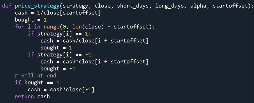
def price_strategy(strategy, close, short_days, long_days, alpha, start_offset):
cash = 1/close[start_offset] # Start with one unit of CCY2, converted into CCY1
bought = 1
for i in range(0, len(close) - start_offset):
#print(strategy[i])
if strategy[i] == 1:
cash = cash/close[i + start_offset]
bought = 1
if strategy[i] == -1:
cash = cash*close[i + start_offset]
bought = -1
# Sell at end
if bought == 1:
cash = cash*close[-1]
#if bought == -1:
# cash = cash - close[-1]
return cash
def graph_strategy(close, strategy, short, long, start_offset):
x = list(range(0, len(close) - start_offset))
plt.figure(0)
plt.plot(x, close[start_offset:], label = Name)
plt.plot(x, short, label = "short_av")
plt.plot(x, long, label = "long_av")
buyidx = []
sellidx = []
for i in range(len(strategy)):
if strategy[i] == 1:
buyidx.append(i)
elif strategy[i] == -1:
sellidx.append(i)
marker_height = (1+0.1)*min(close) - 0.1*max(close)
plt.scatter(buyidx, [marker_height]*len(buyidx), label = "Buy", marker="|")
plt.scatter(sellidx, [marker_height]*len(sellidx), label = "Sell", marker="|")
plt.title('Moving average crossover')
plt.xlabel('Timestep')
plt.ylabel('Price')
plt.legend()
def plot_param(x, close, start_offset, param_index, param_values):
profit = []
x2 = x.copy()
for value in param_values:
x2[param_index] = value
short_days = x2[0]
long_days = x2[1]
alpha = x2[2]
threshold = x2[3]
(strat, short, long) = calculate_strategy(close, short_days, long_days, alpha, start_offset, threshold)
profit.append(price_strategy(strat, close, short_days, long_days, alpha, start_offset) - 1)
plt.figure(param_index+1)
param_names = ["short_days", "long_days", "alpha", "threshold"]
name = param_names[param_index]
plt.title('Strategy profit vs ' + name)
plt.xlabel(name)
plt.ylabel('Profit')
plt.plot(param_values, profit, label = "Profit")
def evaluate_params(x, close, start_offset):
short_days = x[0]
long_days = x[1]
alpha = x[2]
threshold = x[3]
(strat1, short, long) = calculate_strategy(close, short_days, long_days, alpha, start_offset, threshold)
profit = price_strategy(strat1, close, short_days, long_days, alpha, start_offset)
return -profit #Since we minimise
#Initial strategy parameters.
short_days = 30
long_days = 300
alpha = 0.95
start_offset = 300
threshold = 0.02#0.01
#short_days = 10marker_height
#long_days = 30
#alpha = 0.75
#alpha = 0.92
#threshold = 0.02
x = [short_days, long_days, alpha, threshold]
#Price strategy
(strat1, short, long) = calculate_strategy(close, short_days, long_days, alpha, start_offset, threshold)
profit = price_strategy(strat1, close, short_days, long_days, alpha, start_offset)
print("Strategy profit is: " + str(profit - 1))
print("Buy and hold profit is: " + str(close[-1]/close[start_offset] - 1))
#Graph strategy
graph_strategy(close, strat1, short, long, start_offset)
#Graph parameter dependence
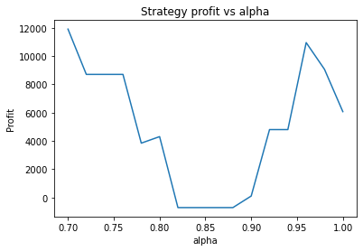
plot_param(x, close, start_offset, 2, np.arange(0.7, 1, 0.02))
plot_param(x, close, start_offset, 3, np.arange(0.01, 0.1, 0.001))
plot_param(x, close, start_offset, 0, np.arange(20, long_days, 10))
plot_param(x, close, start_offset, 1, np.arange(short_days, 300, 10))
The crossing over of short and long term moving averages is a well-known signal used in algo trading. The idea is that when the short term average rises above the long term average, it could indicate the price is beginning to rise. Similarly, when the short term average falls below the long term average, it could indicate the price is beginning to fall. The Binance academy refers to these as the golden cross and death cross respectively. Moving averages can be applied to Bitcoin or other cryptocurrencies as a strategy or one component of a strategy.
The moving average strategy has a number of parameters that need to be determined:
short_days – The number of days used for the short term average
long_days – The number of days used for the long term average
alpha – This is a parameter used in the exponential moving average calculation which determines how much less weight is given to data further in the past. A value of 1 means all data gets the same weighting.
threshold – A threshold of 10% means that instead of executing when the two averages cross, we require that the short average pass the long average by 10%. The idea is to prevent repeatedly entering/exiting a trade if the price is jumping about near the crossover point.
Of course, one can also consider combining moving averages with other signals/strategies like pairs trading to improve its effectiveness.
In this article we create python code to backtest a moving average crossover strategy on historical bitcoin spot data from Binance.
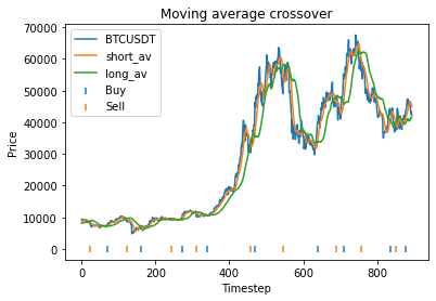
We grab the daily Binance BTCUSD close spot prices for the past 945 days here. The data ranges from September 2019 to April 2022. For our purposes we will ignore the complexities introduced by the order book, and assume there is always enough liquidity at the top of the book for the quantity we want to trade. This will likely be the case for individual investors trading their own money, for example. We will also ignore transaction costs, since these are usually negligible compared to price changes unless we are examining a high frequency strategy.
The full python code is included at the bottom of this post. It features the following functions:
moving_avg – This computes a moving average a number of days before a given index. The function was modifed to accept non-integer number of days in case it needed to work with an optimization algorithm.
calculate_strategy – This takes as input the strategy parameters and calculates where the strategy buys/sells.
price_strategy – This takes the strategy created by calculate_strategy and calculates the profit on this strategy on the current data.
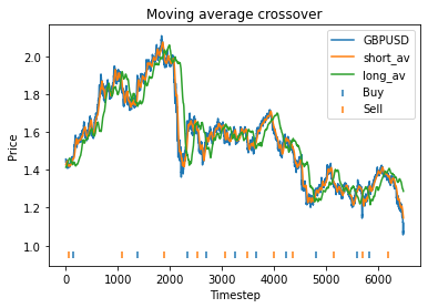
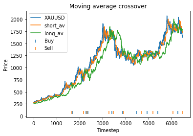
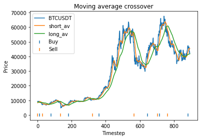
graph_strategy – This generates a graph of the price data, along with the short and long term moving averages and indicators showing where the strategy buys/sells
plot_param – This plots profit as a function of one of the parameters to help gauge optimal values
evaluate_params – This is a reformating of the price_strategy function to make it work with optimization algorithms like scipy.optimize.
We assume that we always either hold or short bitcoin based on whether the strategy predicts that the price is likely to rise or fall. To begin, we choose some initial parameters more or less at random.
Then we execute the code. this produces the following output. This means that using these parameters,
Strategy profit is: 31758.960000000006
Buy and hold profit is: 33115.64
This means that with these randomly chosen parameters, our strategy actually performs slightly worse than simply buying and holding. The code produces this graph which shows the bitcoin price, long and short averages, and markers down the bottom indicating where the strategy decided to buy and sell. It’s apparent that the strategy executes essentially where the orange and green lines crossover (although the threshold parameter mentioned earlier will affect this).
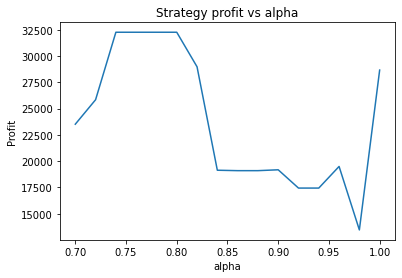
The code also produces the following graphs which show how the strategy profit varies with each parameter.
These graphs are quite “jumpy”, i.e. have a significant amount of noise. An attempt to find the optimal parameters using optimization algorithms would probably just “overfit” to the noise (or just get stuck at a local maximum). It’s clear that to deploy optimization algorithms to find the optimal parameters, you would probably need to apply some kind of multidimensional smoothing algorithm to create a smoother objective function. You could also attempt to use more data, however going back further means the data may become less relevant.
Instead, we proceed using visual inspection only. However, it’s important to realise that these parameters are potentially interdependent so one has to be careful optimizing them one at a time. We could consider looking at three dimensional graphs to get a better idea of what’s going on. From the first plot, it appears that an alpha of 0.92 is optimal. The threshold graph is very jumpy, but it appears as if the graph has an overall downward trend. Thus we choose the threshold to be a small value, say 0.02. The short averaging days graph also has a downward trend, so let’s make it something small like 10. The long averaging days graph indicates that the strategy performs poorly for smaller values. Let’s try making it 35. Now let’s run the code again with these new parameters.
Strategy profit is: 41372.97999999998
Buy and hold profit is: 33115.64
So our strategy is now more profitable than buy and hold, at 41.4k vs 33.1k.
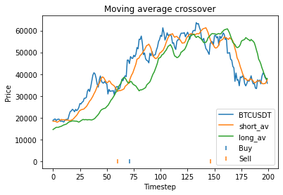
Our optimized strategy has performed considerably better than our initial choice of parameters, and considerably better than buy and hold. But before we get excited, we have to consider the possibility that we have overfitted. That is, we have found parameters that perform exceptionally on this particular dataset, but may perform poorly on other datasets (particular future datasets). One way to explore this question is to break the data up into segments and run the code individually on each segment to see whether the optimal parameters disagree. Let’s try to 400 to 600 region from the graph first.
Strategy profit is: 32264.25
Buy and hold profit is: 17038.710000000003
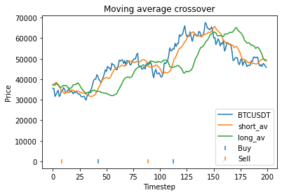
In this region, the strategy is still dramatically more profitable than buy and hold, and an alpha of 0.75 still seems to be approximately optimal. Now let’s look at the region from 600 to 800 on the original graph.
Strategy profit is: 8708.76000000001
Buy and hold profit is: 10350.419999999998
In this region, the strategy actually performs worse than buy and hold (although the loss is massively outweighed by the profit from the 400 to 600 region). While an alpha of 0.75 still seems approximately optimal, the strategy doesn’t perform significantly better than buy and hold for any value of alpha.
Below is the full python code used to fit the strategy and create the graphs used in this article. The four parameters can be manually altered under “initial strategy parameters”.
import numpy as np
import pandas as pd
import matplotlib.pyplot as plt
from scipy.optimize import minimize
data = pd.read_csv("Binance_BTCUSDT_d.csv")
data = data.iloc[::-1] #reverses order of dates
close = np.array(data.close)
def moving_avg(close, index, days, alpha):
# float values allowed for days for use with optimization routines.
partial = days - np.floor(days)
days = int(np.floor(days))
weights = [alpha**i for i in range(days)]
av_period = list(close[max(index - days + 1, 0): index+1])
if partial > 0:
weights = [alpha**(days)*partial] + weights
av_period = [close[max(index - days, 0)]] + av_period
return np.average(av_period, weights=weights)
def calculate_strategy(close, short_days, long_days, alpha, start_offset, threshold):
strategy = [0]*(len(close) - start_offset)
short = [0]*(len(close) - start_offset)
long = [0]*(len(close) - start_offset)
boughtorsold = 1
for i in range(0, len(close) - start_offset):
short[i] = moving_avg(close, i + start_offset, short_days, alpha)
long[i] = moving_avg(close, i + start_offset, long_days, alpha)
if short[i] >= long[i]*(1+threshold) and boughtorsold != 1:
boughtorsold = 1
strategy[i] = 1
if short[i] <= long[i]*(1-threshold) and boughtorsold != -1:
boughtorsold = -1
strategy[i] = -1
return (strategy, short, long)
def price_strategy(strategy, close, short_days, long_days, alpha, start_offset):
cash = -close[start_offset] # subtract initial purchase cost
bought = 1
for i in range(0, len(close) - start_offset):
#print(strategy[i])
if strategy[i] == 1:
# Note the factor of 2 is due to selling and shorting
cash = cash - 2*close[i + start_offset]
bought = 1
if strategy[i] == -1:
cash = cash + 2*close[i + start_offset]
bought = -1
# Sell at end
if bought == 1:
cash = cash + close[-1]
if bought == -1:
cash = cash - close[-1]
return cash
def graph_strategy(close, strategy, short, long, start_offset):
x = list(range(0, len(close) - start_offset))
plt.figure(0)
plt.plot(x, close[start_offset:], label = "BTCUSDT")
plt.plot(x, short, label = "short_av")
plt.plot(x, long, label = "long_av")
buyidx = []
sellidx = []
for i in range(len(strategy)):
if strategy[i] == 1:
buyidx.append(i)
elif strategy[i] == -1:
sellidx.append(i)
plt.scatter(buyidx, [0]*len(buyidx), label = "Buy", marker="|")
plt.scatter(sellidx, [0]*len(sellidx), label = "Sell", marker="|")
plt.title('Moving average crossover')
plt.xlabel('Timestep')
plt.ylabel('Price')
plt.legend()
def plot_param(x, close, start_offset, param_index, param_values):
profit = []
x2 = x.copy()
for value in param_values:
x2[param_index] = value
short_days = x2[0]
long_days = x2[1]
alpha = x2[2]
threshold = x2[3]
(strat, short, long) = calculate_strategy(close, short_days, long_days, alpha, start_offset, threshold)
profit.append(price_strategy(strat, close, short_days, long_days, alpha, start_offset))
plt.figure(param_index+1)
param_names = ["short_days", "long_days", "alpha", "threshold"]
name = param_names[param_index]
plt.title('Strategy profit vs ' + name)
plt.xlabel(name)
plt.ylabel('Profit')
plt.plot(param_values, profit, label = "Profit")
def evaluate_params(x, close, start_offset):
short_days = x[0]
long_days = x[1]
alpha = x[2]
threshold = x[3]
(strat1, short, long) = calculate_strategy(close, short_days, long_days, alpha, start_offset, threshold)
profit = price_strategy(strat1, close, short_days, long_days, alpha, start_offset)
return -profit #Since we minimise
#Initial strategy parameters.
short_days = 15
long_days = 50
alpha = 1
start_offset = long_days
threshold = 0.05
#short_days = 10
#long_days = 30
#alpha = 0.75
#alpha = 0.92
#threshold = 0.02
x = [short_days, long_days, alpha, threshold]
#Price strategy
(strat1, short, long) = calculate_strategy(close, short_days, long_days, alpha, start_offset, threshold)
profit = price_strategy(strat1, close, short_days, long_days, alpha, start_offset)
print("Strategy profit is: " + str(profit))
print("Buy and hold profit is: " + str(close[-1] - close[start_offset]))
#Graph strategy
graph_strategy(close, strat1, short, long, start_offset)
#Graph parameter dependence
plot_param(x, close, start_offset, 2, np.arange(0.7, 1, 0.02))
plot_param(x, close, start_offset, 3, np.arange(0.01, 0.1, 0.001))
plot_param(x, close, start_offset, 0, np.arange(5, long_days, 1))
plot_param(x, close, start_offset, 1, np.arange(short_days, 50, 1))
#Optimization
#x0 = [short_days, long_days, alpha, threshold]
#start_offset = 70
#bnds = ((1, start_offset), (1, start_offset), (0.001,1), (0,None))
#cons = ({'type': 'ineq', 'fun': lambda x: x[1] - x[0]})
#result = minimize(evaluate_params, x0, args=(close, start_offset), bounds=bnds, constraints=cons, method='BFGS')
#print(result)
#evaluate_params(result.x, close, start_offset)
Are you interested in developing an automated algorithm to trade on Interactive Brokers? Have a successful strategy already that you want automated in order to monitor a large number of data streams? Want your strategy backtested and optimized? We offer algorithmic trading consulting services for Interactive Brokers, including: algorithm implementation in python or C++, data analysis, backtesting and machine learning. Please get in touch to learn more!
About Interactive Brokers
Interactive Brokers is a large US-based brokerage firm dealing in stocks, ETFs, options, bonds and forex. Since 2021, it also offers cryptocurrency spot and futures trading.
Initial setup
Although Interactive Brokers also supports C#, C++, Java and VB, most people will probably prefer the convenience of python unless they are doing high frequency trading or their strategy is computationally demanding.
Of course, the first step is always to open an account with the broker which you can do here.
Getting setup to do algo trading on Interactive Brokers requires a few more steps than many other brokers. You’ll need to download and install their python API and their Trader Work Station app (TWS). The latter must be running in the background while you run your algo from your favourite python IDE.
After creating an ordinary account with Interactive Brokers, TWS gives you the option to log in with a paper trading account to allow you to test your algo code without making live trades. Paper accounts (otherwise known as test or demo accounts) usually have the limitation that the order book is not simulated, so they are useful for testing your code and learning how to use the API, but not always for evaluating the profitability of your strategy.
Before trying to connect using your python IDE, make sure “Enable ActiveX and Socket Clients” is ticked under File > Global Configuration > API > Settings.
Python initialization
The next step is to start reading IB’s API documentation to learn about the functionality.
These are some import statements you want at the beginning of your code:
from ibapi.client import EClient from ibapi.wrapper import EWrapper from ibapi.contract import Contract from ibapi.order import Order
And these statements will initialize the connection to the broker.
app = IBapi() app.connect(‘127.0.0.1’, 7497, 123)
The number 7497 is the socket port which can be found in the API settings in TWS mentioned above. The client ID can be an arbitrary positive integer. The EClientSocket class is used to send data to the TWS application, while the EWrapper interface is used to receive data from the TWS application.
Historical and streaming data
Using Interactive Broker’s API is slightly more complicated than for some other exchanges. As they explain in the API documentation here, the EWrapper interface needs to be implemented/overwritten by you to specify what should happen with data you request. So certain functions in the IBapi class will need to be implemented/overwritten to send the data where you want it to go. For example, to request historical data, I like to overwrite the historicalData function like this:
def grab_historical_data(): data = [] app.reqHistoricalData(1, eurusd_contract, ”, ’90 D’, ‘1 day’, ‘MIDPOINT’, 0, 2, False, []) return data
This will grab daily price data for the last 90 days. It appears to use business days rather than calendar days. The interval of 90 days is calculated from the prior day’s close, so the last datapoint should be yesterday’s. Note that each day’s data contains open, close, high and low values. The variable eurusd_contract is actually a contract object which we’ll explain shortly.
If instead of getting historical data you wish to stream the latest price data as it becomes available, you want to overwrite the tickdata function use the function reqMktData as follows.
class IBapi(EWrapper, EClient): def init(self): EClient.init(self, self) def tickPrice(self, reqId, tickType, price, attrib): if tickType == 2 and reqId == 1: print(‘The current ask price is: ‘, price) latest_ask.append(price)
While cryptocurrency exchanges have been offering various kinds of delta one derivatives for a number of years now (such as perpetual futures), the availability of vanilla European call/put options (let alone more complex derivatives) is still nascent. Understandably, traders entering the crypto space would like access to the same tools that they are used to in more traditional and developed markets. Even Goldman Sachs is onboard with the development of a bitcoin options market. Yet, the high volatility of cryptocurrencies produces some unique challenges for the creation of derivatives markets.
Perpetual futures (also called perpetual swaps) on crypto underlyings like Bitcoin are a derivative product first offered by Bitmex and now offered by many cryptocurrency exchanges. Cryptocurrency exchanges typically offer them with up to 100x leverage. While they are similar in some ways to ordinary futures contracts, there are some significant differences.
Firstly, and giving rise to the name, they have no expiry and can instead be closed out at any time by the holder. They could also be closed out by the exchange if the holder gets liquidated, which we’ll discuss shortly.
Secondly there is a mechanism called the funding rate. In an ordinary futures market, the futures price is always related to the spot price. This is ensured by the fact that the futures price converges to the spot price as time approaches the expiry. Since a perpetual futures market has no expiries, this characteristic, if desired, must be created artificially. The funding rate is set by the exchange and is used to ensure the futures price does not diverge too far from the spot market. It is paid directly between market participants and not to the exchange. When the futures price is above the index price, the rate is positive, and traders long perpetual futures must pay the funding rate to those who are short. When the futures price is below the index price, the rate is negative, shorts must pay longs. Note that the index price here could be a weighted average of the spot price among multiple exchanges. In many cases the funding rate is paid every eight hours.
Perpetual options are similar to perpectual futures, except that one replaces the futures payoff with that of a call option or put option. See our main article on perpetual options.
Liquidation
The high volatility of cryptocurrencies combined with the high leverage offered by many exchanges creates challenges for the operation of margin accounts. Because of this, crypto exchanges tend to liquidate positions well before the participants actually run out of margin. If they are able to close out the position at better than the bankruptcy price, this extra money goes into an insurance fund. This is a buffer the exchange uses to ensure it is able to pay traders who have profited from price moves.
Options – calls and puts
Cryptocurrency exchanges are increasingly interested in branching out into options. While some exchanges already offer versions of European and American call/put options, other exchanges are rapidly trying to develop them. More exotic options such as barrier options and Asian options will presumably become common eventually.
It’s well-known that vanilla option prices increase with increasing volatility. This is because higher volatility means increased upside potential, yet the holder is protected from the increased downside risk by the optionality. Thus crypto options are expected to have considerably higher premiums than those on equity or FX markets.
As a few examples of the current options offerings of various exchanges:
Binance offers American options on BTCUSDT futures with expiries from ten minutes up to one day (note that USDT is a cryptocurrency with value tethered to the USD dollar). Binance offers only ATM call and put options, that is, there is only one available strike which is equal to the most recent traded perpetual futures price.
Bitmex does not currently provide options, but is keen to develop this capability.
How to price cyptocurrency options
A reasonable starting point for pricing European options on cryptocurrencies is the Black-Scholes framework. In the case of American options, one can apply the binomial tree method. In either case, all of the pricing parameters such as spot and time to expiry are straight forward to determine except one – the volatility.
As is well-known, in developed options markets including equity, FX and interest rate options, the volatility is not really an input but is inferred from existing market prices. When calculated in this way, the volatility is inconsistent between options of differing strike and expiry, leading to a smile or volatility surface.
However, in the case of a nascent cryptocurrency options market, the market is unlikely to be sufficiently liquid, especially at the beginning, to obtain these market prices. In fact, many crypto exchanges do not allow options to be traded. Instead, the exchange functions as a market maker and simply sets the price itself.
Of course, one can always use an empirical calculation of historical volatility as a starting point, but a smile of some kind would need to be imposed upon it. One way to do this would be to start with the smile for an equity of FX rate which is believed to be in some sense similar to bitcoin, and scale it by a factor determined by taking the ratio of the equity ATM vol with the empirical volatility of the cryptocurrency.
Each exchange (or broker) provides slightly different services and features to traders wishing to automate their strategies as algos.
Some exchanges provide their own high-level trading language allowing people unfamiliar with conventional coding languages to implement and test simple algorithms. I don’t favor this approach as I would rather take advantage of the powerful features of a language like python.
Some exchanges provide a simple API key allowing you to interface with the exchange from you favorite language. Others require that you download additional software in order to interface (and authenticate) with the exchange.
Some exchanges provide a test account allowing you to test your code without having to risk money on live trades
Some exchanges do not allow customers to connect to their API unless they meet certain requirements. For example, TradeStation requires that your account have $10,000 of cash deposited before they will email you your API key. This is very bothersome if you initially intend to just develop and test your algorithm, and only invest your money at an appropriate time in the future.
Here we provide a few exchange specific guides, outlining how to get started interfacing with the exchange, grabbing price histories and posting buy/sell orders:
Are you interested in developing an automated algorithm to trade crypto on Binance? Have a successful strategy already that you want automated in order to monitor a large number of data streams 24/7? Want your strategy backtested and optimized? We offer algorithmic trading consulting services for spot, futures and option trading on Binance, including: trading bot implementation in python or C++, data analysis, backtesting and machine learning. Please get in touch to learn more!
About Binance
Binance is one of the world’s largest cryptocurrency exchanges, offering:
Spot trading on around 100 digital currencies including Bitcoin and Ethereum
Up to 125x leverage on perpetual futures contracts
At the money American call and put options with 5 minute to 1 day expiries
Note that Binance has been banned by regulators in some countries such as the US and the UK due to concerns about the compliance of cryptocurrency exchanges with anti-money-laundering laws (competitor Bitmex is in a similar situation). Binance.US is an alternative which is designed to comply with US regulations.
Crypto exchanges are keen to develop cryptocurrency derivative products such as futures and European or American options. But keep in mind that some countries like Australia, Germany, Italy and the Netherlands only allow trading in spot, as they have banned derivatives including futures, options and leverage. Regulators are concerned that retail investors may be unaware of the risk involved in derivative products given the high volatility of cryptocurrencies.
Initial setup
Since Cryptocurrency markets do not close overnight, algorithmic trading using a crypto bot is the only way to monitor your positions 24/7.
First you need to make sure you have an installation of python. I recommend downloading the Anaconda distribution which comes with the Spyder IDE. In addition, you’ll want the python library python-binance, which can be obtained by opening an anaconda prompt from the start menu and typing
pip install python-binance
In addition, an API key is needed to give your installation of python permission to trade on your binance account. After creating a Binance account, simply go to the profile icon in the top right corner and click “API Management”. Then just place these lines at the top of your python code:
from binance import Client, ThreadedWebsocketManager, ThreadedDepthCacheManager
client = Client(API Key, Secret Key)
Here, API Key and Secret Key are of course the two keys you obtained from Binance.
Backtesting data
Binance market data for backtesting purposes can be downloaded here. Spot and futures data are available with three file types as shown below. As the raw data comes without headers, I’ve included screenshots below showing the headers for convenience.
AggTrades
Klines
Trades
Basic commands to get you started
From there, one can start reading the Binance API to start learning basic commands.
If you want to receive an updated price only when it has changed, you can stream prices by creating a threaded websocket manager. The function “update_price” defines what to do whenever some new information “info” is received from the exchange. In this case it appends it onto a vector of historical prices and prints it out to the console.