In a couple of previous articles, we backtested and optimized a moving average crossover strategy for both Bitcoin and FX.
Now while backtesting on historical data is a key part of developing a trading strategy, it also has some limitations that are important to be aware of.
Firstly you have the issue that you usually have a limited amount of historical data. And even if you could obtain data going back as many years as you wanted, the relevance of older data is questionable. Also, when you have a finite amount of data, there’s always the problem of overfitting. This occurs when we optimize too much for the idiosyncrasies of one particular dataset, rather than trends and characteristics which are likely to be persistant.
And even if you had say, ten years of data, if there happened to be no GFC during those ten years you’d have no idea how the strategy would perform under that scenario. And what about scenarios that have never happened yet? A strategy that is perfectly optimized for historical data may not perform well in the future because there’s no guarantee that future asset and market behaviour will mimic past behaviour.
This is where backtesting using synthetic data comes in.
Synthetic data is data that is artificially generated. It can be generated so as to try to mimic certain properties of a real historical dataset, or it can be generated to test your strategy against hypothetical scenarios and asset behaviour not seen in the historical data.
Now the downside of backtesting using synthetic data is that it may not accurately depict the real behaviour of the asset. However, even real historical data may not be representative of future behaviour.
With synthetic data, one can generate any amount of data, say 100 years or even more. This means:
- No problems with overfitting – you can generate an unlimited amount of data to test whether optimized parameters work in general or only on a specific piece of data.
- The large amount of data should contain a wider range of possible data patterns to test your strategy on.
- Mathematical optimization algorithms for finding optimal parameters work perfectly as they can work with smooth, noise free functions.
- It’s easy to explore how properties of the data (eg, volatility) affect the optimal parameters. This can ultimately allow you to use adaptive parameters for your strategy, which change based on changing characteristics of the data such as volatility.
- It allows you to test how robust your strategy is on hypothetical scenarios that might not have occurred in the historical data. For example, if you backtested your strategy on data with lower volatility, will it still be profitable if the asset volatility increases? Would your strategy be profitable (or at least minimize losses) during a market crash?
How to generate synthetic data
In general, when generating asset paths for stocks, cryptocurrencies or exchange rates, the starting point is geometric Brownian motion. For some applications you may wish to add random jumps to the Brownian motion, the timing of which can be generated from a Poisson process.
However, when generating synthetic data for backtesting purposes you will probably find that your strategy is completely ineffective when applied to geometric Brownian motion alone. This is because real asset price data contains non-random features such as trends, mean reversions, and other patterns which are exactly what algorithmic traders are looking for.
This means that we have add trend effects to our synthetic data. However, it does raise a significant issue: how do we know that the artificial trends and patterns we add to the data are representative of those present in real data?
What you’ll find is that the profitability of the strategy is largely determined by the relative magnitudes of the geometric motion and the trend term. If the trend is too strong, the strategy will be phenomenally profitable. Too weak, and the strategy will have nothing but random noise to work with.
We will not concern ourselves too much with generating highly natural or realistic data in the present article as our primary purpose here is to study how synthetic data can allow us to explore the behaviour of the strategy, and how its optimal parameters relate to the properties of the data.
We generate synthetic FX data using the code below. We assume the initial FX rate is S0 = 1, and volatility is 10%. Since, barring some kind of hyperinflation event, an exchange rate does not usually become unboundedly large or small, we add in some mean reversion that tends to bring it back to its original value.
While there are many ways of defining a trend, our trend is a value which starts at 0 and drifts randomly up or down due to it’s own geometric brownian motion. There is also a mean reversion term which tends to bring the trend back to 0. The trend value is added to the stock jump each time step.
def generate_path(S0, num_points, r, t_step, V, rand, rand_trend, mean, mean_reversion):
S = S0*np.ones(num_points)
trend = 0
for i in range(1, len(S)):
trend = trend + rand_trend[i-1]*S[i-1]/2000 - trend/10
S[i] = mean_reversion*(mean - S[i-1]) + S[i-1]*np.exp((r - 0.5*V**2)*t_step + np.sqrt(t_step)*V*rand[i-1]) + 0.7*trend
return S
# Generate synthetic data
S0 = 1
num_points = 50000
seed = 123
rs = np.random.RandomState(seed)
rand = rs.standard_normal(num_points-1)
rand_trend = rs.standard_normal(num_points-1)
r=0
V=0.1
t_step = 1/365
mean = 1
mean_reversion = 0.004
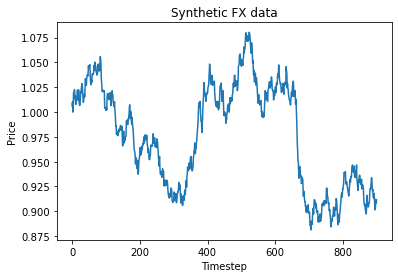
close = generate_path(S0, num_points, r, t_step, V, rand, rand_trend, mean, mean_reversion)To get an idea of what our synthetic data looks like, below I’ve generated and plotted 1000 days of synthetic FX data.
Backtesting an FX moving average strategy on synthetic data
We generate 100,000 days of synthetic FX data and run our moving average backtesting script from the previous two articles.
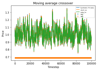
Plotting 100,000 datapoints on a graph along with the short and long moving averages produces a seriously congested graph. However, we can see that the synthetic data does not stray too far from its initial value of 1. In fact, we could probably stand to relax the mean reversion a bit if it was realistic data we were after. The greatest variation from the initial value of 1 seems to be about 30% which is too low over such a long time period. Now the profitability of the strategy is not particularly meaningful here, since as mentioned it is largely determined the strength of the trend as compared to the Brownian motion that the user specifies. If the strategy is profitable, the profit will also be very high when the strategy is executed over 100,000 days.
What is interesting though, is to strengthen the trend of the data (say, changing 0.7*trend to 1*trend in the earlier code snippet) and plotting graphs of profitability vs parameter values. When backtesting against real historical data, we often found that the resulting graphs were noisy and multi-peaked, making it difficult to determine the optimal parameters. Using a much larger quantity of synthetic data with a strong trend, we find the graphs are clean and clear.
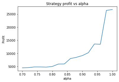
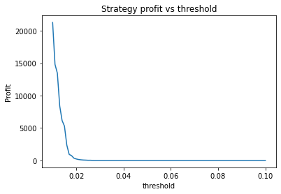
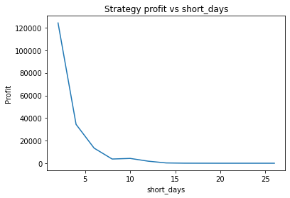
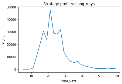
We can clearly see that the optimal values are alpha close to 1, say 0.975, threshold as small as possible, short days also very small and long days about 22.
What happens if we make the volatility of the data smaller by a factor of 3?
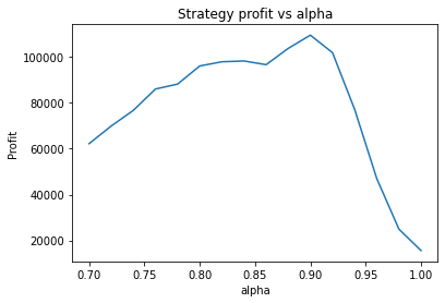
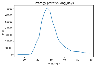
It seems the optimal alpha has reduced to about 0.9. Also, the optimal number of days used for the long term average has increased from low twenties to high twenties.
It’s unlikely you’d be able to extract this insight from backtesting on historical data. Firstly, you wouldn’t be able to adjust the volatility of the data on a whim, and the graphs would be too noisy to clearly see the relationship. What this example illustrates is that synthetic data can be used to study how various properties of the data affect the optimal parameters of the strategy. This could be used to create a strategy with “adaptive” parameters which change based on the most recent characteristics of the data, such as volatility. A very simple example of this would be increasing the number of days used in the long term average during periods of high volatility.
Testing stressed artificial scenarios
Another utility of synthetic data is the ability to generate particular scenarios on which to test your strategy. This might include periods of high volatility, steeply declining or rising data, or sudden jumps. To achieve this, one can generate some synthetic data using the method already described, and then manually adjust the data points to create a particular scenario. This will help you to understand what kind of data may “break” your strategy and how you might be able to adjust parameters, or add in additional conditional behaviour or fail safes.
Find out more about our algorithmic trading consulting services.
Python code
Below we include the python code used to generate the numbers and graphs in this article.
import numpy as np
import pandas as pd
import matplotlib.pyplot as plt
from scipy.optimize import minimize

def generate_path(S0, num_points, r, t_step, V, rand, rand_trend, mean, mean_reversion):
    S = S0*np.ones(num_points)
    trend = 0
    for i in range(1, len(S)):
        trend = trend + rand_trend[i-1]*S[i-1]/2000 - trend/10
        S[i] = mean_reversion*(mean - S[i-1]) + S[i-1]*np.exp((r - 0.5*V**2)*t_step + np.sqrt(t_step)*V*rand[i-1]) + 0.7*trend

    return S

# Generate synthetic data
S0 = 1
num_points = 100000
seed = 123
rs = np.random.RandomState(seed)
rand = rs.standard_normal(num_points-1)
rand_trend = rs.standard_normal(num_points-1)
r=0
V=0.1
t_step = 1/365
mean = 1
mean_reversion = 0.004
close = generate_path(S0, num_points, r, t_step, V, rand, rand_trend, mean, mean_reversion)

def moving_avg(close, index, days, alpha):
    partial = days - np.floor(days)
    days = int(np.floor(days))

    weights = [alpha**i for i in range(days)]
    av_period = list(close[max(index - days + 1, 0): index+1])

    if partial > 0:
        weights = [alpha**(days)*partial] + weights
        av_period = [close[max(index - days, 0)]] + av_period

    return np.average(av_period, weights=weights)

def calculate_strategy(close, short_days, long_days, alpha, start_offset, threshold):
    strategy = [0]*(len(close) - start_offset)
    short = [0]*(len(close) - start_offset)
    long = [0]*(len(close) - start_offset)
    boughtorsold = 1
    for i in range(0, len(close) - start_offset):
        short[i] = moving_avg(close, i + start_offset, short_days, alpha)
        long[i] = moving_avg(close, i + start_offset, long_days, alpha)
        if short[i] >= long[i]*(1+threshold) and boughtorsold != 1:
            boughtorsold = 1
            strategy[i] = 1
        if short[i] <= long[i]*(1-threshold) and boughtorsold != -1:
            boughtorsold = -1
            strategy[i] = -1
    return (strategy, short, long)

def price_strategy(strategy, close, short_days, long_days, alpha, start_offset):
    cash = 1/close[start_offset]  # Start with one unit of CCY2, converted into CCY1
    bought = 1
    for i in range(0, len(close) - start_offset):
        if strategy[i] == 1:
            cash = cash/close[i + start_offset]
            bought = 1
        if strategy[i] == -1:
            cash = cash*close[i + start_offset]
            bought = -1
    # Sell at end
    if bought == 1:
        cash = cash*close[-1]
    return cash

def graph_strategy(close, strategy, short, long, start_offset):
    x = list(range(0, len(close) - start_offset))
    plt.figure(0)
    plt.plot(x, close[start_offset:], label = "Synthetic FX data")
    plt.plot(x, short, label = "short_av")
    plt.plot(x, long, label = "long_av")
    buyidx = []
    sellidx = []
    for i in range(len(strategy)):
        if strategy[i] == 1:
            buyidx.append(i)
        elif strategy[i] == -1:
            sellidx.append(i)
    marker_height = (1+0.1)*min(close) - 0.1*max(close)
    plt.scatter(buyidx, [marker_height]*len(buyidx), label = "Buy", marker="|")
    plt.scatter(sellidx, [marker_height]*len(sellidx), label = "Sell", marker="|")
    plt.title('Moving average crossover')
    plt.xlabel('Timestep')
    plt.ylabel('Price')
    plt.legend(loc=1, prop={'size': 6})
    #plt.legend()

def plot_param(x, close, start_offset, param_index, param_values):
    profit = []
    x2 = x.copy()
    for value in param_values:
        x2[param_index] = value
        short_days = x2[0]
        long_days = x2[1]
        alpha = x2[2]
        threshold = x2[3]
        (strat, short, long) =  calculate_strategy(close, short_days, long_days, alpha, start_offset, threshold)
        profit.append(price_strategy(strat, close, short_days, long_days, alpha, start_offset) - 1)
    plt.figure(param_index+1)
    param_names = ["short_days", "long_days", "alpha", "threshold"]
    name = param_names[param_index]
    plt.title('Strategy profit vs ' + name)
    plt.xlabel(name)
    plt.ylabel('Profit')
    plt.plot(param_values, profit, label = "Profit")

def evaluate_params(x, close, start_offset):
    short_days = x[0]
    long_days = x[1]
    alpha = x[2]
    threshold = x[3]
    (strat1, short, long) =  calculate_strategy(close, short_days, long_days, alpha, start_offset, threshold)
    profit = price_strategy(strat1, close, short_days, long_days, alpha, start_offset)
    return -profit #Since we minimise

#Initial strategy parameters.
short_days = 5
long_days = 30
alpha = 0.99
start_offset = 100
threshold = 0.01

x = [short_days, long_days, alpha, threshold]

#Price strategy
(strat1, short, long) =  calculate_strategy(close, short_days, long_days, alpha, start_offset, threshold)
profit = price_strategy(strat1, close, short_days, long_days, alpha, start_offset)
print("Strategy profit is: " + str(profit - 1))
print("Buy and hold profit is: " + str(close[-1]/close[start_offset] - 1))

#Graph strategy
graph_strategy(close, strat1, short, long, start_offset)

#Graph parameter dependence
plot_param(x, close, start_offset, 2, np.arange(0.7, 1, 0.02))
plot_param(x, close, start_offset, 3, np.arange(0.01, 0.1, 0.001))
plot_param(x, close, start_offset, 0, np.arange(2, long_days, 2))
plot_param(x, close, start_offset, 1, np.arange(short_days, 60, 2))