Our quant consulting service can help you backtest and optimize your moving average strategy. Find out more about our algorithmic trading consulting services and contact us today.
See also our article on backtesting an FX moving average strategy on synthetic data.
Some distinguishing characteristics of Forex trading, as opposed to stock trading, is 24 hour trading, virtually no limit on liquidity, and the potential for significant leverage on trades. These features are all fortuitous for an algorithmic approach to trading.
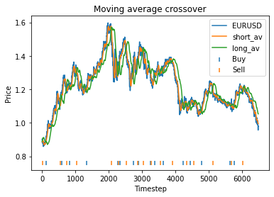
The crossing over of short and long term moving averages is a well-known signal used in algo trading. The idea is that when the short term average rises above the long term average, it could indicate the price is beginning to rise. Similarly, when the short term average falls below the long term average, it could indicate the price is beginning to fall.
In a previous article, we investigated backtesting a moving average crossover strategy on bitcoin. We found that our backtesting allowed us to pick optimal parameters for the strategy that very significantly improved its profitability, and resulted in a far higher return than simply buying and holding the asset.
In this article we conduct the same analysis on four currency pairs – GBPUSD, EURUSD, AURUSD and XAUUSD. Forex data going back to January 2001 has been sourced from forextester.
We assume that the trader initially converts one USD to the other currency, converts back and forth between the two currencies based on whether he believes the exchange rate is trending up or down, and converts back to USD at the end. The profit is compared against that of simply holding the non-USD currency for the entire time.
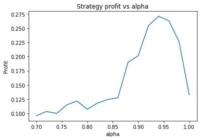
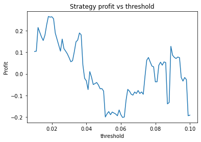
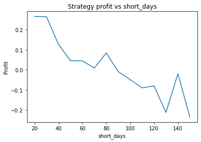
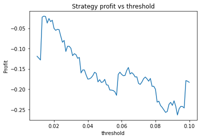
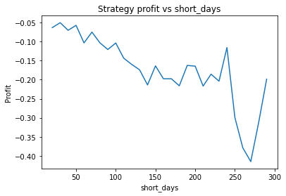
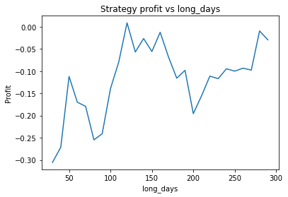
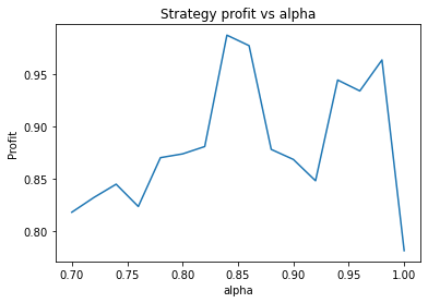
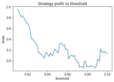
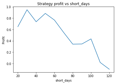
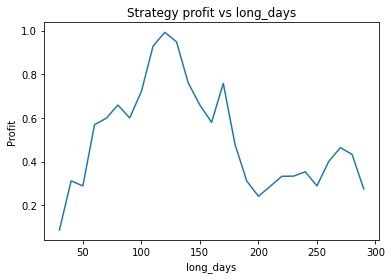
As before our strategy has four parameters to optimize: alpha, threshold, short days and long days.
- short_days – The number of days used for the short term average
- long_days – The number of days used for the long term average
- alpha – This is a parameter used in the exponential moving average calculation which determines how much less weight is given to data further in the past. A value of 1 means all data gets the same weighting.
- threshold – A threshold of 10% means that instead of executing when the two averages cross, we require that the short average pass the long average by 10%. The idea is to prevent repeatedly entering/exiting a trade if the price is jumping about near the crossover point.
We plot graphs showing the profit of the strategy for different values of each parameter. From these graphs, we choose optimal parameters for each currency pair. The full results, graphs and the python code used in this analysis are available below.
Conclusions
There are many pitfalls and caveats when doing this kind of optimization, and what seem like the optimal parameters should never be accepted naively. Things to keep in mind:
- We are finding the optimal parameters on a particular piece of historical data. There is no guarantee that these parameters will be effective on future data which may differ in significant ways from historical data.
- We have to be careful we are not “overfitting”, which occurs when we optimize too much for the idiosyncrasies of our particular dataset, rather than trends which are likely to persist. One way to guard against this is to split the data into pieces and perform the optimization on each piece. This gives an idea of how much variation to expect in the optimal parameters.
A question that arises in our set of graphs below, is how to choose parameters when the graph of profit against parameter value is noisy, multi-peaked or has highly unstable peaks (eg two close together parameters values that have radically different profitability).
We find different currency pairs exhibit differing optimal parameters. However, a critical question is how much of this variation is genuine, and can be expected to hold into the future, and how much is just noise in the data. However, generally speaking we find the following parameters are effective in most cases:
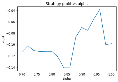
- Alpha large, say 0.95
- Threshold small – 0.01 or 0.02. This indicates that the threshold variable is often not useful and could perhaps be removed.
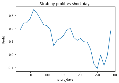
- Short days between 30 and 60
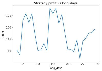
- Long days between 120 and 160
This information is certainly useful, and helps us to configure our moving average strategy much better than if we were merely guessing at, for example, how many days to take the long average over. It’s important to realise that even the most carefully optimized strategy can fail when conditions emerge that were not present in its historical backtesting dataset.
It’s worth noting that these optimal parameters differ from those we found for bitcoin. In that case, we found a long days parameter of just 35 and a short days parameter of just 10 were optimal. This probably reflects the much higher volatility of bitcoin as compared to Forex markets.
This article highlights some of the difficulties involved in backtesting strategies on historical data. One way to resolve many of these issues is to test and optimize your strategy on synthetic data. This will be the subject of a future article.
Results
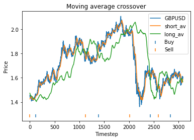
GBPUSD
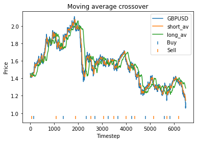
Strategy profit is: 0.2644639031872955
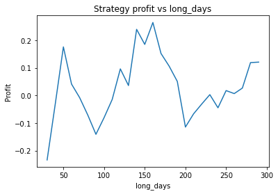
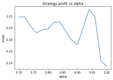
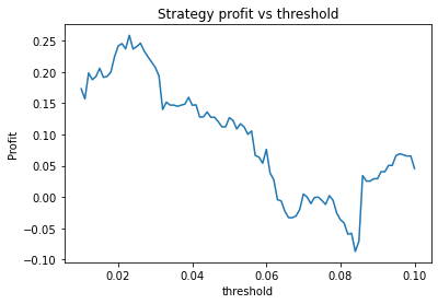
Buy and hold profit is: -0.23343631994507374We find that the optimal alpha is about 0.95. The threshold graph displays a general downward trend so we choose threshold = 0.02. The short days graph displays a clear downward trend so we choose short_days = 30. The long days graph displays a peak at about 160. It’s not entirely clear whether or not this peak is simply an artifact of the particular dataset we are looking at. If we believed this, we might choose a value more like 300 since the graph displays a general upward trend. Regardless, we choose long_days = 160 in this case.
Using these values, our strategy has a profit of 0.26 USD, vs a loss of 0.23 USD from buying and holding GBP.
Another thing we can do here is guard against overfitting by splitting the dataset into two halves, repeat the process on each piece, and seeing whether the optimal parameters change much. Surprisingly, we find that the optimal parameters are about the same for both halves of the data. This will often not be the case, however.
First half:
Second half:
EURUSD
Strategy profit is: 0.9485592864080428
Buy and hold profit is: 0.086715457972943
We choose alpha = 0.95, threshold = 0.01, short_days = 30, long_days = 130.
Using these values, our strategy has a profit of 0.95 USD, vs a profit of 0.087 USD from buying and holding EUR.
AUDUSD
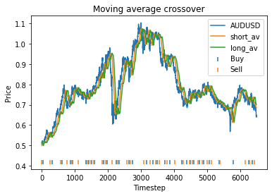
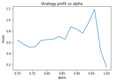
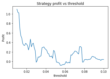
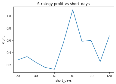
Strategy profit is: 1.0978809301386634
Buy and hold profit is: 0.24194800155219265
From these graphs, it seems an optimal choice of parameters might be apha = 0.95, threshold = 0.01, short_days = 80, long_days = 125. Using these parameters are strategy returns 1.1 USD vs 0.24 USD for buy and hold. However, it’s also clear that the parameters alpha, short_days and long_days are highly unstable. The optimum occurs at a narrow peak, with relatively nearby parameter values giving dramatically lower performance.
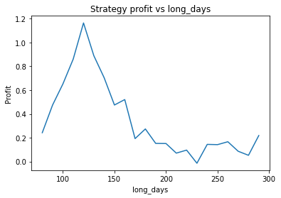
XAUUSD
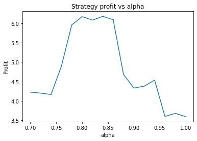
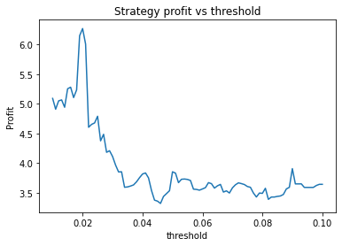
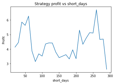
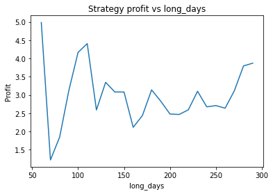
Strategy profit is: 6.267892218264149
Buy and hold profit is: 4.984864864864865
We first try parameters of alpha = 0.85, threshold = 0.02, short_days = 60, long_days = 300. This results in a profit of 6.27 USD versus a buy and hold profit of 4.98 USD.
Interestingly, there is another optimum given by alpha = 0.95, threshold = 0.1, short_days = 60, long_days = 300.
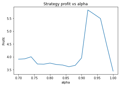
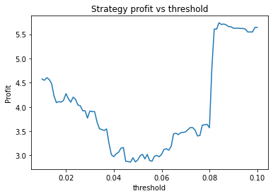
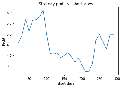
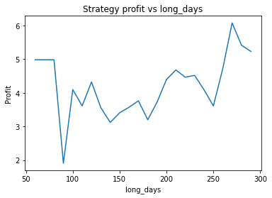
Strategy profit is: 5.640074352374969
Buy and hold profit is: 4.984864864864865
The way the threshold and alpha graphs change when we change the base threshold and alpha shows the interdependence of the parameters.
Python code
The python code used in this analysis is made available below.
import numpy as np
import pandas as pd
import matplotlib.pyplot as plt
from scipy.optimize import minimize
#data = pd.read_csv("GBPUSD.txt")
idx = 0
Names = ["GBPUSD", "EURUSD", "AUDUSD", "XAUUSD"]
Name = Names[idx]
data = pd.read_csv(Name + ".txt")
#data = data.iloc[::-1] #reverses order of dates
# Filter for daily data only
data = data.drop_duplicates(subset=['<DTYYYYMMDD>'], keep='last')
close = np.array(data["<CLOSE>"])
#close = close[:3389]
def moving_avg(close, index, days, alpha):
# float values allowed for days for use with optimization routines.
partial = days - np.floor(days)
days = int(np.floor(days))
weights = [alpha**i for i in range(days)]
av_period = list(close[max(index - days + 1, 0): index+1])
if partial > 0:
weights = [alpha**(days)*partial] + weights
av_period = [close[max(index - days, 0)]] + av_period
return np.average(av_period, weights=weights)
def calculate_strategy(close, short_days, long_days, alpha, start_offset, threshold):
strategy = [0]*(len(close) - start_offset)
short = [0]*(len(close) - start_offset)
long = [0]*(len(close) - start_offset)
boughtorsold = 1
for i in range(0, len(close) - start_offset):
short[i] = moving_avg(close, i + start_offset, short_days, alpha)
long[i] = moving_avg(close, i + start_offset, long_days, alpha)
if short[i] >= long[i]*(1+threshold) and boughtorsold != 1:
boughtorsold = 1
strategy[i] = 1
if short[i] <= long[i]*(1-threshold) and boughtorsold != -1:
boughtorsold = -1
strategy[i] = -1
return (strategy, short, long)
def price_strategy(strategy, close, short_days, long_days, alpha, start_offset):
cash = 1/close[start_offset] # Start with one unit of CCY2, converted into CCY1
bought = 1
for i in range(0, len(close) - start_offset):
#print(strategy[i])
if strategy[i] == 1:
cash = cash/close[i + start_offset]
bought = 1
if strategy[i] == -1:
cash = cash*close[i + start_offset]
bought = -1
# Sell at end
if bought == 1:
cash = cash*close[-1]
#if bought == -1:
# cash = cash - close[-1]
return cash
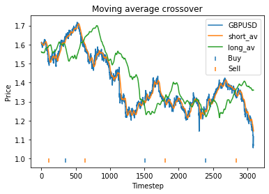
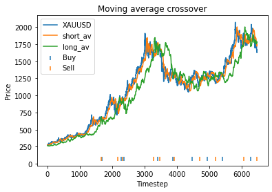
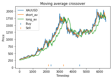
def graph_strategy(close, strategy, short, long, start_offset):
x = list(range(0, len(close) - start_offset))
plt.figure(0)
plt.plot(x, close[start_offset:], label = Name)
plt.plot(x, short, label = "short_av")
plt.plot(x, long, label = "long_av")
buyidx = []
sellidx = []
for i in range(len(strategy)):
if strategy[i] == 1:
buyidx.append(i)
elif strategy[i] == -1:
sellidx.append(i)
marker_height = (1+0.1)*min(close) - 0.1*max(close)
plt.scatter(buyidx, [marker_height]*len(buyidx), label = "Buy", marker="|")
plt.scatter(sellidx, [marker_height]*len(sellidx), label = "Sell", marker="|")
plt.title('Moving average crossover')
plt.xlabel('Timestep')
plt.ylabel('Price')
plt.legend()
def plot_param(x, close, start_offset, param_index, param_values):
profit = []
x2 = x.copy()
for value in param_values:
x2[param_index] = value
short_days = x2[0]
long_days = x2[1]
alpha = x2[2]
threshold = x2[3]
(strat, short, long) = calculate_strategy(close, short_days, long_days, alpha, start_offset, threshold)
profit.append(price_strategy(strat, close, short_days, long_days, alpha, start_offset) - 1)
plt.figure(param_index+1)
param_names = ["short_days", "long_days", "alpha", "threshold"]
name = param_names[param_index]
plt.title('Strategy profit vs ' + name)
plt.xlabel(name)
plt.ylabel('Profit')
plt.plot(param_values, profit, label = "Profit")
def evaluate_params(x, close, start_offset):
short_days = x[0]
long_days = x[1]
alpha = x[2]
threshold = x[3]
(strat1, short, long) = calculate_strategy(close, short_days, long_days, alpha, start_offset, threshold)
profit = price_strategy(strat1, close, short_days, long_days, alpha, start_offset)
return -profit #Since we minimise
#Initial strategy parameters.
short_days = 30
long_days = 300
alpha = 0.95
start_offset = 300
threshold = 0.02#0.01
#short_days = 10marker_height
#long_days = 30
#alpha = 0.75
#alpha = 0.92
#threshold = 0.02
x = [short_days, long_days, alpha, threshold]
#Price strategy
(strat1, short, long) = calculate_strategy(close, short_days, long_days, alpha, start_offset, threshold)
profit = price_strategy(strat1, close, short_days, long_days, alpha, start_offset)
print("Strategy profit is: " + str(profit - 1))
print("Buy and hold profit is: " + str(close[-1]/close[start_offset] - 1))
#Graph strategy
graph_strategy(close, strat1, short, long, start_offset)
#Graph parameter dependence
plot_param(x, close, start_offset, 2, np.arange(0.7, 1, 0.02))
plot_param(x, close, start_offset, 3, np.arange(0.01, 0.1, 0.001))
plot_param(x, close, start_offset, 0, np.arange(20, long_days, 10))
plot_param(x, close, start_offset, 1, np.arange(short_days, 300, 10))