Our quant consulting service can help you backtest and optimize your moving average strategy. Find out more about our algorithmic trading consulting services and contact us today.
See also our article on backtesting a moving average strategy on synthetic data.
The crossing over of short and long term moving averages is a well-known signal used in algo trading. The idea is that when the short term average rises above the long term average, it could indicate the price is beginning to rise. Similarly, when the short term average falls below the long term average, it could indicate the price is beginning to fall. The Binance academy refers to these as the golden cross and death cross respectively. Moving averages can be applied to Bitcoin or other cryptocurrencies as a strategy or one component of a strategy.
The moving average strategy has a number of parameters that need to be determined:
- short_days – The number of days used for the short term average
- long_days – The number of days used for the long term average
- alpha – This is a parameter used in the exponential moving average calculation which determines how much less weight is given to data further in the past. A value of 1 means all data gets the same weighting.
- threshold – A threshold of 10% means that instead of executing when the two averages cross, we require that the short average pass the long average by 10%. The idea is to prevent repeatedly entering/exiting a trade if the price is jumping about near the crossover point.
Of course, one can also consider combining moving averages with other signals/strategies like pairs trading to improve its effectiveness.
In this article we create python code to backtest a moving average crossover strategy on historical bitcoin spot data from Binance.
We grab the daily Binance BTCUSD close spot prices for the past 945 days here. The data ranges from September 2019 to April 2022. For our purposes we will ignore the complexities introduced by the order book, and assume there is always enough liquidity at the top of the book for the quantity we want to trade. This will likely be the case for individual investors trading their own money, for example. We will also ignore transaction costs, since these are usually negligible compared to price changes unless we are examining a high frequency strategy.
The full python code is included at the bottom of this post. It features the following functions:
- moving_avg – This computes a moving average a number of days before a given index. The function was modifed to accept non-integer number of days in case it needed to work with an optimization algorithm.
- calculate_strategy – This takes as input the strategy parameters and calculates where the strategy buys/sells.
- price_strategy – This takes the strategy created by calculate_strategy and calculates the profit on this strategy on the current data.
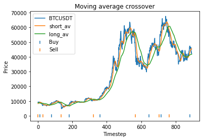
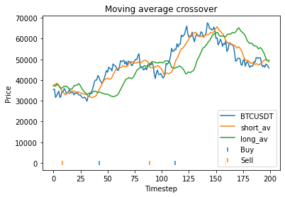
- graph_strategy – This generates a graph of the price data, along with the short and long term moving averages and indicators showing where the strategy buys/sells
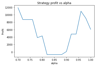
- plot_param – This plots profit as a function of one of the parameters to help gauge optimal values
- evaluate_params – This is a reformating of the price_strategy function to make it work with optimization algorithms like scipy.optimize.
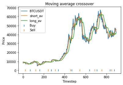
We assume that we always either hold or short bitcoin based on whether the strategy predicts that the price is likely to rise or fall. To begin, we choose some initial parameters more or less at random.
#Initial strategy parameters.
short_days = 15
long_days = 50
alpha = 1
start_offset = long_days
threshold = 0.05
Then we execute the code. this produces the following output. This means that using these parameters,
Strategy profit is: 31758.960000000006
Buy and hold profit is: 33115.64
This means that with these randomly chosen parameters, our strategy actually performs slightly worse than simply buying and holding. The code produces this graph which shows the bitcoin price, long and short averages, and markers down the bottom indicating where the strategy decided to buy and sell. It’s apparent that the strategy executes essentially where the orange and green lines crossover (although the threshold parameter mentioned earlier will affect this).
The code also produces the following graphs which show how the strategy profit varies with each parameter.
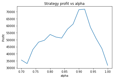
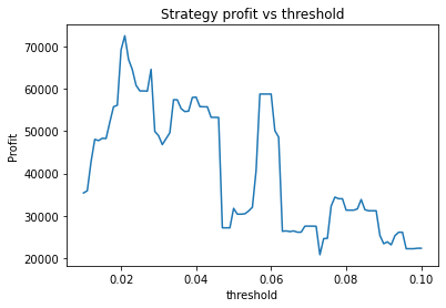
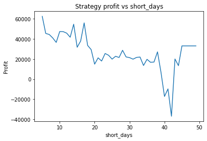
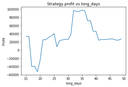
These graphs are quite “jumpy”, i.e. have a significant amount of noise. An attempt to find the optimal parameters using optimization algorithms would probably just “overfit” to the noise (or just get stuck at a local maximum). It’s clear that to deploy optimization algorithms to find the optimal parameters, you would probably need to apply some kind of multidimensional smoothing algorithm to create a smoother objective function. You could also attempt to use more data, however going back further means the data may become less relevant.
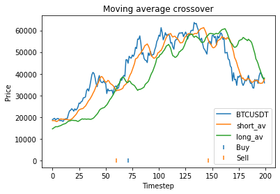
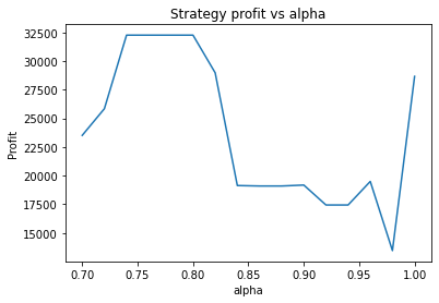
Instead, we proceed using visual inspection only. However, it’s important to realise that these parameters are potentially interdependent so one has to be careful optimizing them one at a time. We could consider looking at three dimensional graphs to get a better idea of what’s going on. From the first plot, it appears that an alpha of 0.92 is optimal. The threshold graph is very jumpy, but it appears as if the graph has an overall downward trend. Thus we choose the threshold to be a small value, say 0.02. The short averaging days graph also has a downward trend, so let’s make it something small like 10. The long averaging days graph indicates that the strategy performs poorly for smaller values. Let’s try making it 35. Now let’s run the code again with these new parameters.
Strategy profit is: 41372.97999999998
Buy and hold profit is: 33115.64
So our strategy is now more profitable than buy and hold, at 41.4k vs 33.1k.
Our optimized strategy has performed considerably better than our initial choice of parameters, and considerably better than buy and hold. But before we get excited, we have to consider the possibility that we have overfitted. That is, we have found parameters that perform exceptionally on this particular dataset, but may perform poorly on other datasets (particular future datasets). One way to explore this question is to break the data up into segments and run the code individually on each segment to see whether the optimal parameters disagree. Let’s try to 400 to 600 region from the graph first.
Strategy profit is: 32264.25
Buy and hold profit is: 17038.710000000003
In this region, the strategy is still dramatically more profitable than buy and hold, and an alpha of 0.75 still seems to be approximately optimal. Now let’s look at the region from 600 to 800 on the original graph.
Strategy profit is: 8708.76000000001
Buy and hold profit is: 10350.419999999998
In this region, the strategy actually performs worse than buy and hold (although the loss is massively outweighed by the profit from the 400 to 600 region). While an alpha of 0.75 still seems approximately optimal, the strategy doesn’t perform significantly better than buy and hold for any value of alpha.
Find out more about our algorithmic trading consulting services.
Also check out our article on statistical arbitrage / pairs trading of cryptocurrency.
Python code
Below is the full python code used to fit the strategy and create the graphs used in this article. The four parameters can be manually altered under “initial strategy parameters”.
import numpy as np
import pandas as pd
import matplotlib.pyplot as plt
from scipy.optimize import minimize

data = pd.read_csv("Binance_BTCUSDT_d.csv")
data = data.iloc[::-1] #reverses order of dates
close = np.array(data.close)

def moving_avg(close, index, days, alpha):
    # float values allowed for days for use with optimization routines.
    partial = days - np.floor(days)
    days = int(np.floor(days))

    weights = [alpha**i for i in range(days)]
    av_period = list(close[max(index - days + 1, 0): index+1])

    if partial > 0:
        weights = [alpha**(days)*partial] + weights
        av_period = [close[max(index - days, 0)]] + av_period

    return np.average(av_period, weights=weights)

def calculate_strategy(close, short_days, long_days, alpha, start_offset, threshold):
    strategy = [0]*(len(close) - start_offset)
    short = [0]*(len(close) - start_offset)
    long = [0]*(len(close) - start_offset)
    boughtorsold = 1
    for i in range(0, len(close) - start_offset):
        short[i] = moving_avg(close, i + start_offset, short_days, alpha)
        long[i] = moving_avg(close, i + start_offset, long_days, alpha)
        if short[i] >= long[i]*(1+threshold) and boughtorsold != 1:
            boughtorsold = 1
            strategy[i] = 1
        if short[i] <= long[i]*(1-threshold) and boughtorsold != -1:
                boughtorsold = -1
                strategy[i] = -1

    return (strategy, short, long)

def price_strategy(strategy, close, short_days, long_days, alpha, start_offset):
    cash = -close[start_offset]  # subtract initial purchase cost
    bought = 1
    for i in range(0, len(close) - start_offset):
        #print(strategy[i])
        if strategy[i] == 1:
            # Note the factor of 2 is due to selling and shorting
            cash = cash - 2*close[i + start_offset]
            bought = 1
        if strategy[i] == -1:
            cash = cash + 2*close[i + start_offset]
            bought = -1
    # Sell at end
    if bought == 1:
        cash = cash + close[-1]
    if bought == -1:
        cash = cash - close[-1]
    return cash

def graph_strategy(close, strategy, short, long, start_offset):
    x = list(range(0, len(close) - start_offset))
    plt.figure(0)
    plt.plot(x, close[start_offset:], label = "BTCUSDT")
    plt.plot(x, short, label = "short_av")
    plt.plot(x, long, label = "long_av")
    buyidx = []
    sellidx = []
    for i in range(len(strategy)):
        if strategy[i] == 1:
            buyidx.append(i)
        elif strategy[i] == -1:
            sellidx.append(i)
    plt.scatter(buyidx, [0]*len(buyidx), label = "Buy", marker="|")
    plt.scatter(sellidx, [0]*len(sellidx), label = "Sell", marker="|")
    plt.title('Moving average crossover')
    plt.xlabel('Timestep')
    plt.ylabel('Price')
    plt.legend()

def plot_param(x, close, start_offset, param_index, param_values):
    profit = []
    x2 = x.copy()
    for value in param_values:
        x2[param_index] = value
        short_days = x2[0]
        long_days = x2[1]
        alpha = x2[2]
        threshold = x2[3]
        (strat, short, long) =  calculate_strategy(close, short_days, long_days, alpha, start_offset, threshold)
        profit.append(price_strategy(strat, close, short_days, long_days, alpha, start_offset))
    plt.figure(param_index+1)
    param_names = ["short_days", "long_days", "alpha", "threshold"]
    name = param_names[param_index]
    plt.title('Strategy profit vs ' + name)
    plt.xlabel(name)
    plt.ylabel('Profit')
    plt.plot(param_values, profit, label = "Profit")

def evaluate_params(x, close, start_offset):
    short_days = x[0]
    long_days = x[1]
    alpha = x[2]
    threshold = x[3]
    (strat1, short, long) =  calculate_strategy(close, short_days, long_days, alpha, start_offset, threshold)
    profit = price_strategy(strat1, close, short_days, long_days, alpha, start_offset)
    return -profit #Since we minimise

#Initial strategy parameters.
short_days = 15
long_days = 50
alpha = 1
start_offset = long_days
threshold = 0.05

#short_days = 10
#long_days = 30
#alpha = 0.75
#alpha = 0.92
#threshold = 0.02

x = [short_days, long_days, alpha, threshold]

#Price strategy
(strat1, short, long) =  calculate_strategy(close, short_days, long_days, alpha, start_offset, threshold)
profit = price_strategy(strat1, close, short_days, long_days, alpha, start_offset)
print("Strategy profit is: " + str(profit))
print("Buy and hold profit is: " + str(close[-1] - close[start_offset]))

#Graph strategy
graph_strategy(close, strat1, short, long, start_offset)

#Graph parameter dependence
plot_param(x, close, start_offset, 2, np.arange(0.7, 1, 0.02))
plot_param(x, close, start_offset, 3, np.arange(0.01, 0.1, 0.001))
plot_param(x, close, start_offset, 0, np.arange(5, long_days, 1))
plot_param(x, close, start_offset, 1, np.arange(short_days, 50, 1))

#Optimization
#x0 = [short_days, long_days, alpha, threshold]
#start_offset = 70

#bnds = ((1, start_offset), (1, start_offset), (0.001,1), (0,None))
#cons = ({'type': 'ineq', 'fun': lambda x:  x[1] - x[0]})

#result = minimize(evaluate_params, x0, args=(close, start_offset), bounds=bnds, constraints=cons, method='BFGS')
#print(result)
#evaluate_params(result.x, close, start_offset)