The relative immaturity of crypto markets may mean there are more opportunities for arbitrage than on more conventional markets. In this article, we investigate whether price moves in crypto coins are correlated. Specifically, we see whether the last three price moves in a selection of coins can be used to predict the next move in a coin of interest. You could consider this strategy to be a type of statistical arbitrage, or a pairs trading strategy (albeit over a small interval of time).
We implement a vector autoregression model on a select of nine major crypto coins, whose tickers are: SOL-USD, BTC-USD, ETH-USD, BNB-USD, XRP-USD, ADA-USD, MATIC-USD, DOGE-USD, DOT-USD. All data is grabbed directly from Yahoo Finance using the yfinance python package. We use one week of data (the most recent at the time of writing) and a 1 minute time interval.
A VAR model is a variety of linear regression that attempts to predict the next move of a particular coin, based on the last few price moves of the coin and all the other coins. The idea is two-fold. Firstly, if two coins tend to correlate but one moves first, it may portend a move of the other coin. Secondly, the VAR model will attempt to find a trend in the coin itself. In fact, a VAR model includes a moving average crossover as a subset of what it can fit. An interesting feature is that it can potentially use moving averages in other coins as a predictive signal. However, I only used the three previous price moves as inputs to the model as using more than this didn’t appear to improve the result in this case.
The results show that the algorithm is effective at predicting the next move of many coins, but does not appear to be effective for bitcoin.
Results
The code produces a scatterplot of the actual vs predicted price moves, along with the correlation and p value between the two. Note that since the code grabs the most recent data at the time of execution, the numbers may differ between runs. Below I show two coins where the algorithm is effective and one where it isn’t.
XRP-USD
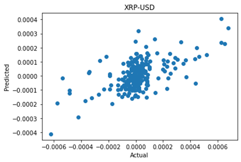
LinregressResult(slope=0.34169299506953943, intercept=2.8755621199597785e-06, rvalue=0.5873282315680474, pvalue=1.551167162089073e-22, stderr=0.031321080004877454, intercept_stderr=5.55906329231313e-06)XRP-USD shows a strong correlation of 0.59 between the actual and predicted next move, with a negligible p value demonstrating statistical significance.
SOL-USD
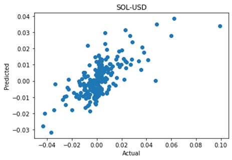
LinregressResult(slope=0.475485553436831, intercept=0.00019601607035287644, rvalue=0.7072734886815194, pvalue=3.3905483806325366e-36, stderr=0.031474953721131224, intercept_stderr=0.0004961483745867841)SOL-USD shows a strong correlation of 0.71, with a negligible p value demonstrating statistical significance.
BTC-USD
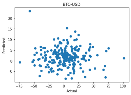
LinregressResult(slope=-0.002493212361084034, intercept=1.8926030981056112, rvalue=-0.015123422722563179, pvalue=0.8195518097975965, stderr=0.010916717835828317, intercept_stderr=0.2832675090566032)By contrast, BTC-USD shows a poor correlation of 0.015 and a p value of 0.8 showing no statistical significance at all. My interpretation of this is that the smaller coins are more likely to be affected by price moves in Bitcoin, rather than the other way around.
For many coins, the algorithm is able to predict the next price move with strong correlation. Thus, the algorithm could be the starting point for an effective strategy for a variety of cryptocoins.
Future development
A good next step for developing this idea would be to explore using a time interval of less than one minute. Particularly in live prediction, one would not want to wait up to a minute to analyse the data and make a decision. Ideally, the algorithm would analyse and take action every time the exchange updated the price of one or more coins. It would also be interesting to develop a model that accesses data for a very large number of assets (including not just crypto but other asset types, economic parameters etc) and search for correlations. One could eventually explore using big data / machine learning techniques to search for these relationships.
Python code
Below is the python code used for this article. You can specify which coin you are trying to predict using the index_to_predict variable. In order to protect against overfitting to a particular piece of historical data, the variable test_fraction specifies how much of the data to set aside for testing (I’ve used the last 20%).
import numpy as np
import pandas as pd
import matplotlib.pyplot as plt
from statsmodels.tsa.api import VAR
from statsmodels.tsa.statespace.tools import diff
from scipy.stats import linregress
import yfinance as yf

# Set data and period interval
period = "1w"
# Valid intervals: [1m, 2m, 5m, 15m, 30m, 60m, 90m, 1h, 1d, 5d, 1wk, 1mo, 3mo]
interval = '1m'

# Number of previous moves to use for fitting
VAR_order = 3

tickers = ["SOL-USD","BTC-USD","ETH-USD","BNB-USD","XRP-USD","ADA-USD","MATIC-USD","DOGE-USD","DOT-USD"]
# Specify which coin to forecast
index_to_predict = 0
test_fraction = 0.2 # fraction of data to use for testing

data = yf.download(tickers = tickers,  # list of tickers
                period = period,         # time period
                interval = interval,       # trading interval
                ignore_tz = True,      # ignore timezone when aligning data from different exchanges?
                prepost = False)       # download pre/post market hours data?

X = np.zeros((data.shape[0],len(tickers)))

for (i,asset) in enumerate(tickers):
    X[:,i] = list(data['Close'][asset])

# Deal with missing data.
NANs = np.argwhere(np.isnan(X))
for i in range(len(NANs)):
    row = NANs[i][0]
    X[row,:] = X[row-1,:]

# Difference data
Xd = diff(X)

# Determine test and fitting ranges
test_start = round(len(Xd)*(1-test_fraction))
Xd_fit = Xd[:test_start]
Xd_test = Xd[test_start:]

model = VAR(Xd_fit)
results = model.fit(VAR_order)
summary = results.summary()
print(summary)

lag = results.k_ar

predicted = []
actual = []
for i in range(lag,len(Xd_test)):
    actual.append(Xd_test[i,index_to_predict ])
    predicted.append(results.forecast(Xd_test[i-lag:i], 1)[0][index_to_predict])

plt.title(tickers[index_to_predict])
plt.scatter(actual, predicted)
plt.xlabel("Actual")
plt.ylabel("Predicted")

print(linregress(actual, predicted))