Need help building a volatility smoothing algorithm? Our quant consulting service can help. Contact us today.
See also our article on generating volatility surfaces from options data in C++.
Implied volatility surfaces and smiles constructed by fitting a cubic spline to raw market data may contain arbitrage. In fact, even if the market data points used do not contain arbitrage, cubic interpolation between data points may introduce it. It is therefore usually desirable to find the best fit of a cubic spline to the data points, under the restriction that the result be arbitrage free. Unlike the basic interpolation approach, the spline need not pass through the data points. This is called volatility smoothing.
There are two kinds of arbitrage on volatility surfaces that we need to guard against:
- Calendar arbitrage. This is where the volatility surface allows a European option with a shorter maturity to be more valuable than an option with a longer maturity, which is impossible (in the absence of dividends). A simple way to see this is to notice that a longer duration has the same effect as a higher volatility, as it gives the volatility more time to act. It’s well-known that higher volatility increases (rather than decreases) the value of the option since it increases the upside but not the downside (since the holder is protected from downside by the strike).
- Butterfly arbitrage. In the strike direction, it’s clear that the price of a call must decrease as the strike increases (more precisely, the first derivative of call price with respect to strike must be less than or equal to zero, with the opposite true for puts). Furthermore, the call price function must be convex, meaning that the second derivative with respect to strike is greater than or equal to zero. To see this, consider selling two calls at strike \(K\), and buying two calls, one at a strike slightly below \(K\), and one at a strike slightly above \(K\). The value of this position is given by the below expression, where \(C\) represents the call price function. It’s easy to see that the payoff at maturity of this position is non-negative. It has value 0 if \(S(T) < K-\Delta K\) or \(S(T) > K+\Delta K\), and positive value otherwise (easy to see by plotting the payoff). By dividing by \(\Delta K\) and taking the limit as \(\Delta K \to 0\), we see that the second derivative must be non-negative.
\[ C(K-\Delta K) – 2C(K) + C(K+\Delta K)\]
\[ = ( C(K+\Delta K – C(K))) – (C(K-\Delta K) – C(K))\]
We recommend the approach of M.R Fengler in his paper Arbitrage-Free Smoothing of the Implied Volatility Surface. Instead of fitting a spline to the graph of volatility vs moneyness, Fengler uses call price vs moneyness. An advantage of this is that the no arbitrage restrictions take on a more simple form in terms of call price.
The surface fitting is done using a least squares fitting, with a number of constraints. The heart of the algorithm is therefore a constrained quadratic optimization procedure. In python, this can be achieved using scipy.optimize.minimise with the parameter method=’SLSQP’. The mathematical difficulty is mainly around understanding the constraints and implementing them accurately.
We’ve implemented Fengler’s algorithm in python. The algorithm runs very quickly on a single vol surface. However, since historical volatility data has, for each date, a large number of vol surfaces (one for each tenor), the number of surfaces to be processed can easily proliferate into the millions. In this case one may wish to consider a C++ implementation or at least a multicore implementation in python.
To illustrate the algorithm, we start with 8 pillar points (moneyness/volatility pairs) which make up the raw data of a vol surface. We’ve deliberately chosen data which contains significant arbitrage. We’ve calculated the Black-Scholes call prices corresponding to these points and plotted them as the blue dots in the below graph.
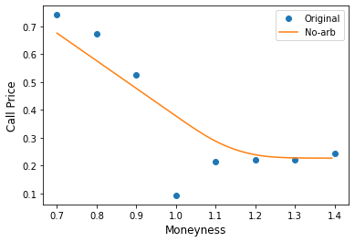
The orange line is the arbitrage free cubic spline generated by our implementation of Fengler’s approach. You can see that it very effectively solves the problem of the out of place at-the-money data point which is entirely inconsistent with an arbitrage free surface.
We can also convert the call prices back to implied volatilities, yielding the following graph. For this graph, we have simply joined the data points by straight lines for illustration purposes.
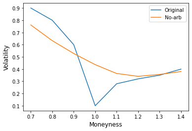
We found we had to make one addition to Fengler’s approach as described in his paper. Fengler considers a set of weights for each data point in the fitting. We found we had to weight each data point by 1/vega to achieve an accurate result. This is because at the wings of the volatility surface, where vega is very small, a small change in call price corresponds to a huge change in volatility. This means that when converting the fitted call prices back to volatilities, the surface will otherwise be a very poor fit in the wings.
Fengler’s paper is not limited to one dimensional volatility surfaces (that is, smiles). It can also be used for two dimensional volatility surfaces which incorporate both moneyness and maturity. His paper details how to extend the method to include maturity.
We provide volatility smoothing consulting, along with a wide range of quantitative finance consulting services.
You may also wish to check out our article on converting volatility surfaces between moneyness and delta.