Genius Mathematics Consultants

Need help building a volatility smoothing algorithm? Our quant consulting service can help. Contact us today.

See also our article on generating volatility surfaces from options data in C++.

Implied volatility surfaces and smiles constructed by fitting a cubic spline to raw market data may contain arbitrage. In fact, even if the market data points used do not contain arbitrage, cubic interpolation between data points may introduce it. It is therefore usually desirable to find the best fit of a cubic spline to the data points, under the restriction that the result be arbitrage free. Unlike the basic interpolation approach, the spline need not pass through the data points. This is called volatility smoothing.

There are two kinds of arbitrage on volatility surfaces that we need to guard against:

• Calendar arbitrage. This is where the volatility surface allows a European option with a shorter maturity to be more valuable than an option with a longer maturity, which is impossible (in the absence of dividends). A simple way to see this is to notice that a longer duration has the same effect as a higher volatility, as it gives the volatility more time to act. It’s well-known that higher volatility increases (rather than decreases) the value of the option since it increases the upside but not the downside (since the holder is protected from downside by the strike).
• Butterfly arbitrage. In the strike direction, it’s clear that the price of a call must decrease as the strike increases (more precisely, the first derivative of call price with respect to strike must be less than or equal to zero, with the opposite true for puts). Furthermore, the call price function must be convex, meaning that the second derivative with respect to strike is greater than or equal to zero. To see this, consider selling two calls at strike \(K\), and buying two calls, one at a strike slightly below \(K\), and one at a strike slightly above \(K\). The value of this position is given by the below expression, where \(C\) represents the call price function. It’s easy to see that the payoff at maturity of this position is non-negative. It has value 0 if \(S(T) < K-\Delta K\) or \(S(T) > K+\Delta K\), and positive value otherwise (easy to see by plotting the payoff). By dividing by \(\Delta K\) and taking the limit as \(\Delta K \to 0\), we see that the second derivative must be non-negative.

\[ C(K-\Delta K) – 2C(K) + C(K+\Delta K)\]

\[ = ( C(K+\Delta K – C(K))) – (C(K-\Delta K) – C(K))\]

We recommend the approach of M.R Fengler in his paper Arbitrage-Free Smoothing of the Implied Volatility Surface. Instead of fitting a spline to the graph of volatility vs moneyness, Fengler uses call price vs moneyness. An advantage of this is that the no arbitrage restrictions take on a more simple form in terms of call price.

The surface fitting is done using a least squares fitting, with a number of constraints. The heart of the algorithm is therefore a constrained quadratic optimization procedure. In python, this can be achieved using scipy.optimize.minimise with the parameter method=’SLSQP’. The mathematical difficulty is mainly around understanding the constraints and implementing them accurately.

We’ve implemented Fengler’s algorithm in python. The algorithm runs very quickly on a single vol surface. However, since historical volatility data has, for each date, a large number of vol surfaces (one for each tenor), the number of surfaces to be processed can easily proliferate into the millions. In this case one may wish to consider a C++ implementation or at least a multicore implementation in python.

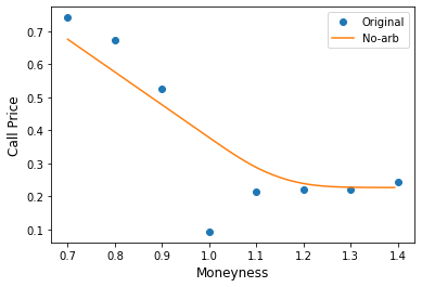
To illustrate the algorithm, we start with 8 pillar points (moneyness/volatility pairs) which make up the raw data of a vol surface. We’ve deliberately chosen data which contains significant arbitrage. We’ve calculated the Black-Scholes call prices corresponding to these points and plotted them as the blue dots in the below graph.

The orange line is the arbitrage free cubic spline generated by our implementation of Fengler’s approach. You can see that it very effectively solves the problem of the out of place at-the-money data point which is entirely inconsistent with an arbitrage free surface.

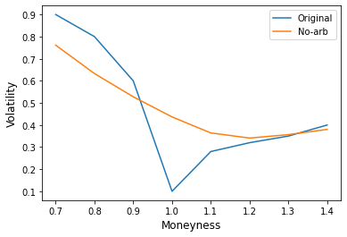
We can also convert the call prices back to implied volatilities, yielding the following graph. For this graph, we have simply joined the data points by straight lines for illustration purposes.

We found we had to make one addition to Fengler’s approach as described in his paper. Fengler considers a set of weights for each data point in the fitting. We found we had to weight each data point by 1/vega to achieve an accurate result. This is because at the wings of the volatility surface, where vega is very small, a small change in call price corresponds to a huge change in volatility. This means that when converting the fitted call prices back to volatilities, the surface will otherwise be a very poor fit in the wings.

Fengler’s paper is not limited to one dimensional volatility surfaces (that is, smiles). It can also be used for two dimensional volatility surfaces which incorporate both moneyness and maturity. His paper details how to extend the method to include maturity.

We provide volatility smoothing consulting, along with a wide range of quantitative finance consulting services.

You may also wish to check out our article on converting volatility surfaces between moneyness and delta.

\(\)It’s well-known that vanilla option valuation does not depend on the term structure of volatility and interest rates. This means that the price depends only on the average volatility and average interest rate between the valuation date and maturity, not on how those quantities are distributed within the interval.

A way to visualize this and understand it intuitively is as follows. Consider a large set of paths of the underlying which have been generated by a Monte Carlo routine. The value of the option is the average over all paths of the quantity \(Max(S(T) – K, 0)\). Now, imagine stretching and compressing the paths in different places as if they were plasticine, corresponding to concentrating volatility more in some places than others. It’s as if the underlying were moving faster in some regions, and slower in others, yet \(S(T)\) remains the same for each path. Thus, the price remains the same.

Interest rates affect the underlying’s drift term. Yet, as for volatility, \(S(T)\) depends only on the total proportional increase that the drift term bestows on the underlying, not on where in the interval this increase occurs.

What about barrier options? There are a few cases to consider.

First, we consider the case of a full barrier option. This means that the barrier is monitored for the full length of the deal from the valuation date to maturity, as opposed to only being monitored for a subset of it. We also assume that the underlying’s drift term is zero (this typically occurs when interest rates are zero, for example). In this case, valuation is actually still independent of volatility term structure. This can be understood by realizing that stretching or compressing the paths in different places does not change whether they breach the barrier, but only when they breach the barrier. Thus whether a given path has knocked-in or knocked-out remains unchanged.

Next, we consider the case of a partial or window barrier option. This means that the barrier is only monitored some of the time, with the monitoring period starting after the valuation date and/or ending before maturity. We still assume that the underlying drift is zero. As mentioned above, while a different volatility term structure does not change whether a path breaches the barrier, it does change when it does. Thus, it can affect whether the path breaches the barrier inside the monitoring window or outside, thus changing whether the path knocks in/out or not. Thus, for partial and window barrier options, valuation is not independent of volatility term structure.

Finally, let’s consider the case of a non-zero drift term. In this case, valuation is not independent of volatility or interest rate term structure regardless of whether it is a full barrier option or a partial/window barrier option. To understand this, consider that the movements in the underlying due to volatility are proportional to the current underlying price. If the underlying is monotonically drifting upwards throughout the monitoring window, then volatility applied early on will cause smaller changes in the underlying than if they were applied towards the end of the monitoring window. Thus, if the volatility term structure concentrates volatility towards the end of the interval after the underlying has had time to drift upwards, they are more likely to cause the underlying to rise above an upper barrier. Thus, volatility term structure and interest rate term structure affect knock out / knock in probability and thus affect valuation.

GPS satellites and receivers are being applied in a huge number of industries including aviation, agriculture, financial fraud identification, robotics (navigation), and landscape surveying.

Developing software to process GPS data requires an understanding of the mathematics involved in GPS coordinate systems, including coordinate transformations between latitude/longitude/height and ECEF coordinates. GPS data often must be combined with other sensor data and run through a mathematical calculation to produce the required output data or system behaviour.

Our consultants can assist you in formulating the correct mathematical equations for your GPS application, and implement them in a variety of languages like python or C++.

While GPUs were originally invented for image processing, their powerful capabilities are now being applied to computation problems that have nothing to do with graphics. As GPUs have about 20x as many cores as CPUS, they can be up to 100x faster for highly parallelizable computations such as machine learning and data analysis.

Did you know that google has used Nvidia GPUs to train its google translate machine learning algorithms?

In particular, Nvidia GPUs find many applications in the financial services industry, which is increasingly making use of massive data sets and AI / deep learning. GPU computation is ideal for Monte Carlo simulations, used extensively in the finance industry, as each path can be processed independently and simultaneously.

CUDA is a program development environment from Nvidia which allows users to execute the highly parallelizable part of their code on an Nvidia GPU.

\(\)It often comes up in quantitative finance that you want to convert a vol surface plotted against moneyness, to a vol surface plotted against delta.

See Options, Futures and Other Derivatives by John Hull for a reference on pricing formulas for European options. In the Black-Scholes framework, the delta of a call option is given by

\[\Delta = N(d_1), \]

Where \(N\) represents the cumulative normal probability density function, and

\[d_1 = \frac{\log(S_0/K) + (r + \sigma^2/2)T}{\sigma \sqrt{T}}. \]

(for a put, it is \(\Delta = N(d_1) – 1 )\) . Rearranging for moneyness, we have

\[ \frac{S_0}{K} = \exp\left(N^{-1}(\Delta) \sigma \sqrt{T} – (r + \sigma^2/2)T \right). \]

Now, our volatility surface would typically be specified using a number of moneyness and volatility pairs \((m_i,v_i)\) where the moneyness values would typically be something like

\[ \{m_i\} = \{0.7, 0.8, 0.9,1,1.1,1.2,1.3\}. \]

When calling for a volitility value for a moneyness in between these numbers, the firm would have implemented an interpolation function,

\[I: \text{ moneyness} \to \text{ volatility},\]

which would typically use a monotonic cubic spline. Inverting this function may be a lot of work, as it would require working out the exact coefficients generated by the cubic spline fitting. Even with an explicit formula, the spline is defined piecewise, which makes inverting it complicated.

Given some delta \(\Delta\) , we want to find a volatility \(\sigma\) such that the moneyness corresponding to that volatility according to the cubic spline interpolation is the same as the moneyness from the above formula. This requires solving the following equation for moneyness \(m\):

\[ m = \exp\left(N^{-1}(\Delta) I(m) \sqrt{T} – (r + I(m) ^2/2)T \right). \]

An equation like this should be solved numerically. This is doubly true due to the complicated definition of the function \(I\). While inverting \(I\) would be difficult, evaluating it is easy. This motivates solving using fixed point methods which only require the function to be evaluated.

What we are looking for is a fixed point of the map \(f\) , i.e. a point \(m\) such that \(f(m) = m\). Thus, in the remainder of the article, we’ll look at an iterative fixed point method for solving this equation. The idea is simple. We start with some initial point \(m_0\), and repeatedly apply the map

\[ f(m) = \exp\left(N^{-1}(\Delta) I(m) \sqrt{T} – (r + I(m) ^2/2)T \right) \]

until the change in \(m\) is less than some small tolerance.

The critical questions is: under what circumstances does this iterative procedure actually converge?

According to the Banach fixed-point theorem, this process will converge to a unique fixed point if \(f\) is a contraction mapping, which in the context of a real-valued function means

\[|f(m_1) – f(m_2)| \leq L |m_1 – m_2|, \]

for some constant \(L \in [0,1)\). This is also known as the Lipschitz condition, and it is well known that

\[L = \sup_m |f'(m)|, \]

where the supremum is of course taken over the domain of interest. Thus, our procedure will converge if \(|f'(m)|<1.\) We calculate,

\[ f'(m) = f(m) I'(m) \left( N^{-1}(\Delta) \sqrt{T} – I(m)T \right). \]

Numerical evidence shows that this derivative does not in general have an absolute value smaller than one, but typically does after just one iteration of our map. Our experience is that this method will almost always converge for all “reasonable” volatility surfaces, and usually within only 2 or 3 iterations!

A possible alternative to searching for a fixed point is to use Newton’s method to search for a zero of the function \(F(m) = m – f(m).\)

\(\)An order imbalance occurs when the buy volume significantly exceeds the sell volume in the order book, or vice versa. They are often caused by news of a significant development that is perceived to affect the value of the stock. It is well-known that order imbalances are an effective predictor of future stock price movement. If demand to buy exceeds the available liquidity, the price will likely move up. If demand to sell is too high for the interest on the buy side to absorb, the price will likely fall. Thus, anyone engaging in algorithmic trading will want to develop algorithms that respond effectively to imbalance signals.

A reasonable definition of order imbalance is

\[ I = \frac{V_b – V_a}{ V_b + V_a },\]

where \(V_b\) and \(V_a\) are the best (or L1) bid and ask volumes. Alternatively, and depending on the application, these volumes may be defined to include multiple levels of the limit order book (a machine learning algorithm would be well suited to determining the complicated relationship between the volume at different levels and the most probable price movement).

A simple approach is described in the book High Frequency Trading by Easley et al. The authors define a “microprice” quantity as a weighted average of the bid and ask price by

\[P_\text{micro} = P_b \frac{V_a}{V_a + V_b} + P_a \frac{V_b}{V_a + V_b}, \]

where \(P_b\) and \(P_a\) are the best (or L1) bid and ask prices, and \(V_b\) and \(V_a\) are the corresponding L1 volumes. The micro price will be closer to the bid price if there is higher volume on the ask side, and closer to the ask price if there is higher volume on the bid side. They then propose to cross the spread on a buy order when \(P _\text{micro}\) is sufficiently close to the ask price, i.e.,

\[P_\text{micro} > P_a – k(P_a – P_b), \]

and analogously for a sell order. Here, \(k\) is some constant specifying the tolerance, which would have to be determined by some kind of tick data analysis technique such as machine learning.

In the book Algorithmic and High Frequency Trading by Cartea et al. the authors discuss a Markov chain approach to modelling the order imbalance. To discretise the problem, order imbalance values are placed into five buckets. A transition matrix is fitted to data. The transition matrix represents the probability of being in each of the five buckets at the next time step, given the current bucket. They also generate data showing the probability of positive and negative price moves based on the current order imbalance bucket.

Are you looking for model validation consulting or advisory services? Our PhD quants have you covered! We provide model validation and model creation consulting services to the financial services industry including banks, hedge funds and trading firms. Contact us to learn more.

Mathematicians have an ability to think clearly and precisely that is rare among finance professionals. We’re excellently placed to provide model validation consulting services. Learn how I found a critical conceptual error in risk modelling work by one of the largest financial consulting firms in the world.

There are two main kinds of models that quantitative analysts are called on to validate in the financial services: derivative pricing models, and risk models.

Validating derivative pricing models

Much of derivative pricing theory is now pretty standard and well-worn. However, there are some choices to be made when validating the appropriateness of the choice of model.

Firstly, there’s the choice of whether to use a computationally slower but more accurate numerical model (such as Monte Carlo, local volatility or stochastic volatility), vs a fast but approximate analytical model. This choice arises with Asian option, where a fast analytic method is known (method of moments), but makes the assumption that the sum of lognormal distributions is lognormal (which is not actually true). Similarly, there exist analytic Black-Scholes formulae for pricing barrier options. However, these models assume that volatility and interest rates are constant. Since volatility term structure has a huge impact on the valuation of barrier options, these models sacrifice a lot of accuracy for speed and simplicity. Whether the trade off is worth it can depend on whether the model is being used to risk purposes (such as a market risk VaR calculation), or front office pricing.

Another issue that arises is the choice of volatility input. Since exotic options are typically not liquid enough to allow for the construction of an implied volatility surface, the use of the European volatility surface must be justified somehow.

Once a model is chosen, there is often no question, in principle, of how to price the derivative. Validating derivative pricing models is thus often mainly about checking the correctness of the coding implementation. A standard way to do this is to build a second, independent model against which to compare the output of the original model. Since it’s impossible to run the two models with all possible inputs, usually one would try to generate a set of test parameters which cover every significant discrete case, such as each possible ordering of date parameters and date coincidence. Another important step is to compare the behaviour of the model to the product description, as just because the two models agree does not necessarily mean they are correctly implementing the intent in the product description. Another important step is to check boundary cases, such as pricing very close to a barrier, very far from a barrier, or after knock-out/knock-in (in the case of barrier options).

An important step is checking the model under stressed scenarios, including very low or very high volatility, and near-zero or negative rates.

However, not all derivatives can be priced with a well-known and standard method. Monte Carlo and other numerical models can require careful work to ensure the model is converging correctly under all circumstances. Custom derivatives can arise which require some ingenuity to price. Examples like high-dimensional derivatives with a large number of underlying assets can require novel mathematics to price, as standard methods are simply not fast enough on current computer hardware. In some cases, pricing early exercise optionality is mathematically non-trivial and/or computationally challenging. As mathematicians, we’re excellently placed to help you price these bespoke derivatives.

See also our derivative pricing consulting services.

Validating risk models

We can build and validate financial risk models including operational risk, market risk and credit risk.

In some cases such as market risk, there are industry standard methodologies (see also our market risk consulting services). However, there are still key choices to be made such as whether to use filtered historical simulation, where data may be weighted by recentness, or adjusted for volatility. One must also decide whether to use absolute or relative shifts, what historical period to use for shift generation, and what time horizon to use for shifts (eg 1 day or 10 day).

For market risk calculations for fixed income products, conceptual pitfalls can arise around calculating shifts in credit spreads (eg bond Z spread). These kinds of subtleties are often missed by the major financial consulting firms, who lack the rigorous mathematical thinking required to detect these errors.

In other cases, such as operational risk, there is no standard approach and much more room for creativity.

Looking for an external model validation consultant? Please get in touch to discuss how we can meet your needs.

Financial derivative valuation requires advanced mathematical skills, coding ability, and financial experience.

Whether you’re looking for a single algorithm or sizable software development, we offer professional cloud-based PhD derivative pricing consulting and advisory services, including

• Equity derivatives
• FX / Forex derivatives
• Interest rate derivatives
• Asian options, barrier options, local volatility models and exotic derivatives
• Bitcoin and cryptocurrency derivatives
• Calculation of equity and interest rate volatility surfaces from market data
• Calculation of greeks including delta, gamma, vega and theta.

We write code scripts or design derivative valuation software to price everything from vanilla options to the exotic derivatives, including:

• Vanilla Black-Scholes for calls and puts
• Forwards and futures
• Interest rate derivatives like swaps, caps and floors
• Local volatility and stochastic volatility models
• American options and exotic options with callability or early exercise optionality
• SABR models
• Fixed interest derivatives like bond futures
• Derivatives on baskets
• Knock in / knock out barrier options and window barrier options. See our article about barrier options and volatility/interest rate term structure. Also, be sure to see the paper by KS Moon for improving the efficiency of Monte Carlo pricing using a Brownian bridge.
• Fixed and variable coupons
• Warrants
• Pnotes (promissory notes)
• Dividend futures

We use a variety of derivative pricing methods including Monte Carlo, Black-Scholes, Finite Difference, and Longstaff-Schwartz. For interest rate derivatives, see the SABR volatility model.

Also check out our article on converting volatility surfaces from moneyness to delta using an iterative procedure.

Need a cloud-based PhD quant to solve all of your derivative pricing problems? Contact us today!

Use the power of Mathematics and Statistics to backtest and optimize your trading strategies against historical data.

Automate your trading strategies with C++/python code to interact directly with the exchange

Ask us how our PhD consultants can help you utilize AI and machine learning in your trading strategies.

Do you have an idea for a trading strategy, but want to prove that it will work through backtesting against historical data? Or do you have a successful trading strategy but want to optimize the parameters of the strategy to maximise returns?

Or perhaps you’ve heard about machine learning and would like to find out how you could incorporate it into your trading. Machine learning can be used to trawl through large amounts of data looking for statistically significant signals to use in your trading. It can also be used to determine the optimal way to combine a number of possible signals or ideas into a single algorithm.

We provide cloud-based PhD quant support for traders. We offer trading algorithm development services for equity and FX markets on all major exchanges. We also offer bitcoin and cryptocurrency algorithmic trading services on major exchanges like Binance and Bitmex.

Our consulting services for algorithmic trading include:

• Backtesting of strategies, strategy optimization and statistical analysis
• Automating algorithms (trading bots) in languages like C++ and python
• Applying machine learning techniques like neural networks to trading
• Processing and analysis of large amounts of data to search for trading signals.
• Pricing of vanilla and exotic derivatives
• Mathematical and statistical research projects
• General quantitative analysis – see our main page Quant Consulting.

Individual traders and smaller financial institutions may lack the quantitative expertise to design or implement trading algorithms, which involves elements of coding, mathematics, statistics and data analysis. Quantitative finance is a field where complex mathematics thrives, so that even sizable firms may wish to undertake projects which are beyond their in-house mathematical expertise. In particular, many firms are interested in dipping their feet into machine learning trading techniques, but lack the necessary internal resources.

Our staff of experienced mathematical researchers can solve sophisticated quantitative problems efficiently, and communicate the results clearly to professionals of all backgrounds. We specialize in advanced mathematical and statistical analysis, and we love a challenge! We can explain and implement the results of sophisticated academic papers and turn them into practical outcomes for your business.

Want to learn more about how cloud-based quant support can supercharge your trading? Contact us today for a frank discussion about the merits of quantitative (or algorithmic) trading.

For examples of the applications of algorithms to trading, see our article on optimal execution algorithms, our article on market making, or our article on algorithms to take advantage of order imbalances.

If you’re just getting started with algorithmic trading, check out our introductory guides to algo trading on various exchanges.

For some examples of backtesting and optimizing trading strategies, take a look at the following articles.

• Backtesting and optimizing a moving average crossover strategy on Bitcoin
• Backtesting and optimizing a moving average strategy on FX markets
• Backtesting algo trading strategies using synthetic data
• Statistical arbitrage / pairs trading on cryptocurrency

Our PhD quant consulting service can canvass the academic literature on trade execution modelling for you, and help you design, backtest and optimize your execution strategy. Contact us to let us know how we can supercharge your trading.

Individual investors who only trade in small volumes may not need to consider an execution strategy. But institutional investors who wish to trade a large number of shares, such as investment banks, hedge funds and mutual funds, encounter the issue that large trades cause adverse price movements. If they attempt to trade the whole amount in one go, liquidity will thin out and they’ll quickly move through less and less favorable bid/ask levels in the limit order book. For this reason, traders will often attempt to split large orders into a series of smaller trades over a period of time. But there are trade offs to a more passive execution strategy. Firstly, there is the opportunity risk that prices will move unfavorably before you liquidate the whole order. Secondly, other traders may notice what you are doing and react accordingly.

Electronic exchanges typically make available not just the best bid and ask prices for a given security, but several layers of bid and ask prices along with the corresponding volumes. This data, known as “market microstructure”, is exactly what we need to inform algorithmic trading algorithms which attempt to optimize execution.

In this article, we’ll explore some of the mathematics around algorithms which optimize execution strategies.

Simple execution models

We first discuss two simple and well-known approaches to order execution, before examining more sophisticated approaches.

TWAP, or Time Weighted Average Price, involves splitting an order into equally sized pieces that are equally spaced in time. When breaking the order into N pieces to be executed over a time T, a fraction 1/N of the order is executed every 1/T seconds. The idea is that the liquidity in the market has time to recover in between orders, avoiding slippage. The price achieved is simply the average of the N prices at each execution.

VWAP, or Volume Weighted Average Price, also breaks the order up into multiple orders spaced at regular time intervals. It differs from TWAP in that the amount transacted at each time step is weighted according to the relative trading volume. Relative trading volume must be judged by using an average over many days in the historical data, and one must assume that the daily trading pattern is persistent. The price achieved is then a weighted average of the N prices at each execution.

POV, or Percentage of Volume, is similar to VWAP except that instead of using historical average volume, the volume over the last say, ten minutes is used. This has a clear advantage if today’s volume could differ substantially from the historical average.

One could improve on both VWAP and POV by both making use of today’s volume data, while still incorporating the historical volume trend to allow you to forecast volume later in the day. More precisely, at each time step the amount remaining to be traded would be apportioned using the most recent volume data for that time step, and the historical forecasted volume for the future timesteps. To get even more fancy, you could try to adjust the historical forecast based on the actual volume traded thus far today – a machine learning algorithm would be great here.

However, the main advantage of these three models is in their simplicity. They are not generally optimal, and their application can potentially be detected by other market participants.

More complex models

A good place to start in exploring more sophisticated execution models is the Almgren-Chriss model. While the model relies on some data that may be difficult to know in practice, it illustrate some of the key issues that should be understood when developing your own personal strategy. See our article on optimal liquidation using the Almgren-Chriss model.

Optimal execution as an optimal stopping problem

The problem of optimally executing a large trade can be cast as one of a familiar class of problems in mathematics – optimal stopping problems.

• Optimal stopping problems in mathematics are are a category of problems where, at any time \(t\), you can choose to “stop”, and receive a certain reward which changes with time. The trouble is you only know what the reward is for the current time and earlier times. You do not know what the reward will be in the future. Should you “cash in your chips” now, or wait, and hope the reward will be better in the future?

The relevance to finance here is obvious. Choosing when to execute trades or exercise an American option are both examples of optimal stopping problems.

Optimal execution using stochastic control theory

In the book Algorithmic and High Frequency Trading by Cartea et al., the authors describe the use of stochastic optimal control and stopping methods to attack this problem.

• Control theory is a field of mathematics that has applications to a wide range of engineering problems. Abstractly, the concept is to find a given “input” to a dynamical system to achieve a desired “output” from the system. A simple example is cruise control, in which the throttle (system input) must be dynamically adjusted to achieve the desired constant speed (system output), for example, when the car begins going uphill. In the case of finance, the dynamical system is typically a stock price \(S(t)\) (typically assumed to follow geometric Brownian motion) or other market information, the system input is the choice of trading strategy, and the system output is the profit of the market participant. The goal is to choose the strategy or “input” which maximises profit.
• Stochastic control theory is a subfield of control theory in which the time evolution of the dynamical system is not completely determined by the system input, but also contains a stochastic or probabilistic element. Financial applications of control theory obviously fall squarely into this category, since market behaviour such as stock prices are not determined solely by the actions of a single market participant, but have a very significant random element.

Finding an optimal strategy or algorithm for market interaction is a problem the arises across a wide range of trading and investing problems. Many of these problems can be cast as stochastic control problems.

Optimal execution using machine learning

Another possible approach to the optimal execution problem is to put to one side attempts to find an optimal theoretical solution, and allow algorithms to trawl through the vast quantities of freely available data and try to determine an effective strategy empirically.

The primary function of such an algorithm would be in estimating the likely shape of the order book. Optimal execution strategies depend critically on how trade volume is distributed among different bid/ask levels. This is because it is this that determines how fast the price will move as you liquidate increasing amounts of inventory. Since the order book data may often be unknown or partial, various machine learning approaches could be effective in developing an empirical model of the order book. The algorithm would analyse how past trades of various sizes affected the top of the order book (taking into account, of course, how closely spaced the trades were in time).

Machine learning is increasingly in vogue in a wide range of fields, including finance. See this useful summary of a report issued by J.P.Morgan about the future of data science and big data in the financial services industry.

In their paper Reinforcement Learning for Optimized Trade Execution, Nevmyvaka et al. examine the effectiveness of machine learning in finding effective execution strategies. See also the more recent paper Double Deept Q-Learning for Optimal Execution by Ning et al.

The execution strategy to be optimized will take as input, at regular time intervals \(t_i\) for \(i=0,\ldots,n\) , a set of observable market variables (principally market microstructure). It produces as output a limit order, or ask price, at which we are willing to execute all remaining inventory. The algorithm may not wait around forever for the best possible price – so it is reasonable to assume that there is a maximum time \(t_n = T\) at which all remaining inventory must be executed regardless of market prices.

By taking a large number of different stocks, and by considering the same stock at different times, we have a large number of data sets of the form \(S(t_i)\) for \(i=0,\ldots,n\). Our execution strategy must depend on time, because as we near the end of the interval, we are running out of time to transact the remaining inventory. As mentioned in the paper by Nevmyvaka, it’s reasonable to make the Markovian assumption that the optimal strategy depends only on market microstructre at the current time step, and not on what it may have been at previous time steps. Thus, whether proceeding by machine learning or by some other method, determining the optimal execution strategy for each step can be done by working backwards from the final time step, in a similar manner to how one prices an American option using Monte Carlo. At time \(t_n = T\) we already know what the strategy is – we must execute all remaining shares regardless of market prices. At time \(t_{n-1}\), for each individual data set we would like to execute at time \(t_{n-1}\) any shares that can be executed at a price equal or better than they could be at time \( T \). The machine learning algorithm must determine, on average after considering all the data sets, what is the optimal map from the market microstructure (bid/ask levels and volumes) to a price at which we are willing to transact at that time step. Continuing to work backwards, we eventually come up with an optimal strategy at each step.

The question remains – what kind of relationship should we assume between the market microstructure and the optimal transaction price at the same time step? We might, with some careful thought, make a guess as to the form of the mathematical function, so that the machine learning algorithm can optimize the parameters. Another option is to use a neural network which may succeed in finding the form of the relationship by itself. Experience shows that making little effort and expecting a machine learning algorithm to work magic is not always successful. Guiding the process using human theoretical insight and human empirical observation, and then using machine learning techniques to merely to optimize, will often yield the best results.