Interested in pricing callable or early exercise derivatives using the Longstaff-Schwartz method? Our consulting service can design and implement a Longstaff-Schwartz algorithm to meet your specific needs, in languages like C++ and python. Learn more about our derivative pricing consulting services.
\(\)In this article we’ll make some interesting observations concerning the well-known Longstaff-Schwarz method for pricing derivatives. Specifically, we’ll look at how to determine an optimal function fitting or regression approach. Most interestingly, we’ll see that one can actually do away with function fitting altogether (!) and apply machine learning and optimization techniques in its place.
In the famous paper of Longstaff and Schwarz, the authors introduced an approach for pricing derivatives that allow for early exercise using Monte Carlo. This includes a vanilla American option and also more complicated exotic options. Their method dramatically reduces the number of paths required by assuming that the relationship between the value of the underlying (or underlyings) and the expected value of continuing (that is, not exercising yet) can be described by a smooth function. In their original paper, they illustrated their method by fitting a quadratic polynomial. This raises the question of what function fitting method should actually be used. What order polynomial should be chosen? Should a more sophisticated non-parametric fitting method be chosen which doesn’t require knowing in advance what kind of function to choose?
We’ll start with a brief recap of the Longstaff-Schwarz method.
Consider pricing an a American call option with expiry \(T\). At any earlier time \(t_0\), the value of exercising the option depends on the current underlying asset price as shown in the following graph.
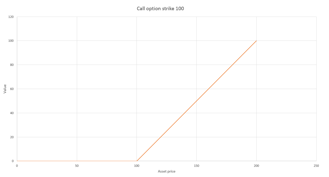
This graph also gives you the fair price of the option at expiry \(T\). We consider that the option can be exercised at a set of time steps \(t_0, t_1, t_2,…,t_n = T\).
Since Longstaff-Schwartz is a Monte Carlo method, we begin by generating a large number of possible future paths for the underlying asset. We can price the option by finding the average payoff over all the asset paths. The complexity comes from the possibility of early exercise, which requires that we determine where it is optimal to exercise for each path. Once we know at which time step a given path will be exercised, the payoff for that path is simply the exercise value at the time step where it is exercised.
- Assuming a given path reaches time \(t_n = T\) without being exercised, it is trivial to determine whether we will exercise based on whether the price is above the strike price or not.
- At \(t_{n-1}\), we assume the option has not yet been exercised, and we have to determine whether to exercise at this step for each path. To do this we compare the value of exercising at this step with the expected value of not exercising
- We can iterate the procedure to determine whether we will exercise earlier at time \(t_{n-2}\). Continuing to iterate, we eventually get back to \(t_0\), having determined for each path the earliest time step where it is optimal to exercise.
So pricing a derivative with early exercise comes down to determining, for each path, the expected value of continuing at each time step.
In the graph below, each blue dot represents one of the paths at some given time step \(t_i\). The horizontal axis shows the payoff from exercising at this time step, and the vertical axis shows the value of continuing based on the known future trajectory of the path. This is the value of exercising at the earliest future time step where we have determined that it is optimal to exercise. But since we wouldn’t normally know the asset path at future time steps, we need to work out the expected value of continuing.
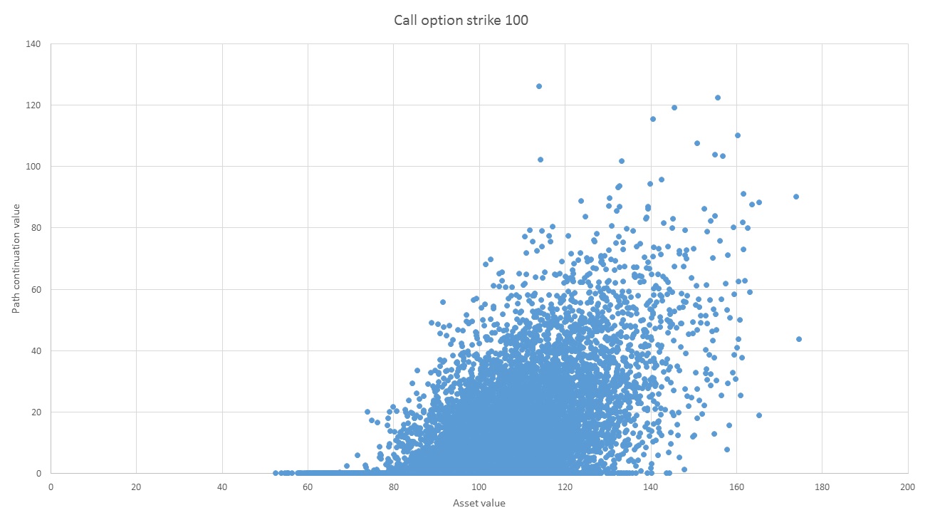
An obvious way to do this would be to generate, for each path above, a large number of future trajectories for that path to find the expected value of continuing. But then the number of paths would grow exponentially at each time step.
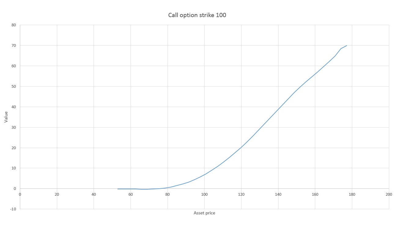
The insight of Longstaff and Schwartz was that we can assume that the expected value of continuing is a smooth function of the asset price. This function can be found using some kind of function fitting or regression technique on the data in the above graph. It turns out that the least squares fitting of a set of vertical points is exactly their average. This means that regression can be viewed as a kind of average which is able to utilize paths at nearby x-values, so we do not need an inordinate number of points vertically above every asset value. The graph below shows a function fitted to the data above.
In their original paper, Longstaff and Schwartz considered using least squares to fit a simple polynomial to the data. However, the literature on function fitting is vast, and a practitioner needs to consider which method to adopt. Since a function must be fitting at each of a potentially large number of time steps, the computational efficiency of the method becomes important. This becomes even more critical when one considers the multidimensional case for basket options with more than one underlying. In this case, we must fit a function of multiple variables. Of course, one also then encounters the curse of dimensionality.
Polynomial fitting has a number of drawbacks. Firstly, a polynomial may not be the appropriate choice for some data sets. Second, you have to decide in advance what order polynomial to choose. If the order is too low, the function will not be able to fit the data. If the order is too high, it suffer from overfitting.
Another approach is to use non-parametric regression methods. For example, local linear regression fits a polynomial only locally, using only points within some “bandwidth” to do the fitting. The fitting can also be weighted so that points further away have less contribution. This is the method used to generate the graph above. However, determining an appropriate bandwidth does give rise to a similar issue to the polynomial case. If the bandwidth is too large, you will miss important function features. Too small, and you will overfit.
The efficacy of different function fitting techniques, particularly non-parametric techniques, is an interesting question. And in considering this question one would examine both the accuracy and the computation time of these methods. But as we’ll see in this article, in considering this one is lead to an even more interesting question – do we need to fit a function at all? Can we simply use optimization and machine learning techniques to determine when it is optimal to exercise?
To see why, let’s start by placing the value of exercising and the our fitting function representing the value of continuing on the same graph.
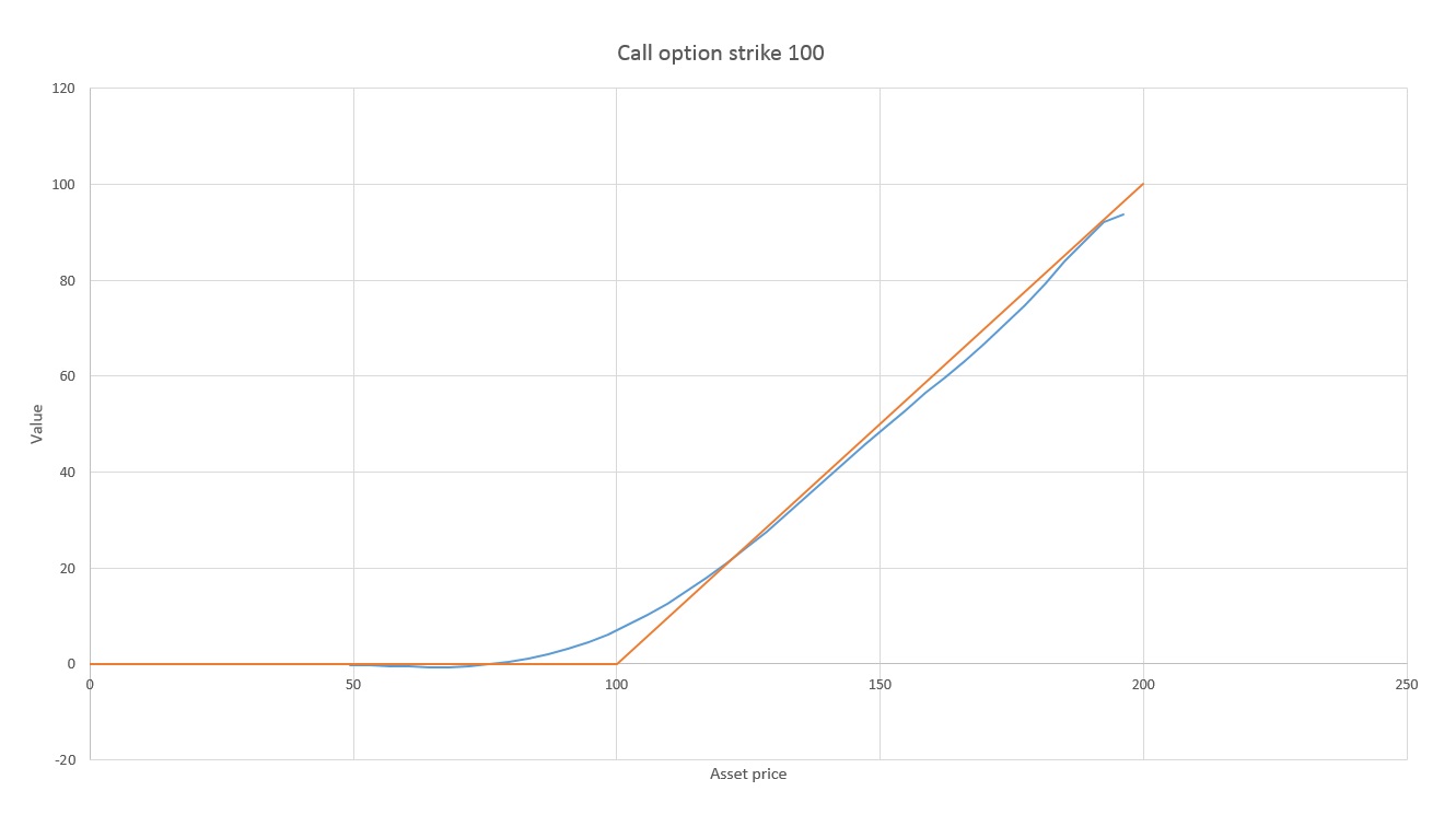
Remember that the only piece of information used in pricing is whether we are going to exercise at this time step. This in turn depends only on whether the fitted function, representing the expected value of continuing, is above or below the exercise value. In the above graph, if the asset has price around 100, it is optimal to continue (not exercise). But once the asset price passes about 122, a slightly higher average payoff comes from exercising now rather than continuing. Thus, if we know that the value of continuing is above the value of exercising on the left hand side, and “crosses over” at about 122, then we have all the information we need to price the option. The exact shape of the blue fitted function is entirely irrelevant beyond that.
This raises a very interesting question. Do we need to fit a function at all?
In the graph below, we introduce a new function labelled “linear fit”. This is a straight line that has been determined using an optimization method. Precisely, for our candidate function \(f(x)\), we have maximised the sum over all paths \(p_i = (x_i,y_i)\) of the following:
\[V(f) = \left\{\begin{array}{lr} y_i, & \text{if } f(x_i) > E(x_i)\\ E(x_i), & \text{if } f(x_i) \leq E(x_i) \end{array}\right\} \]
Here, \(E(x)\) is the function representing the value of exercising for asset price \(x\).
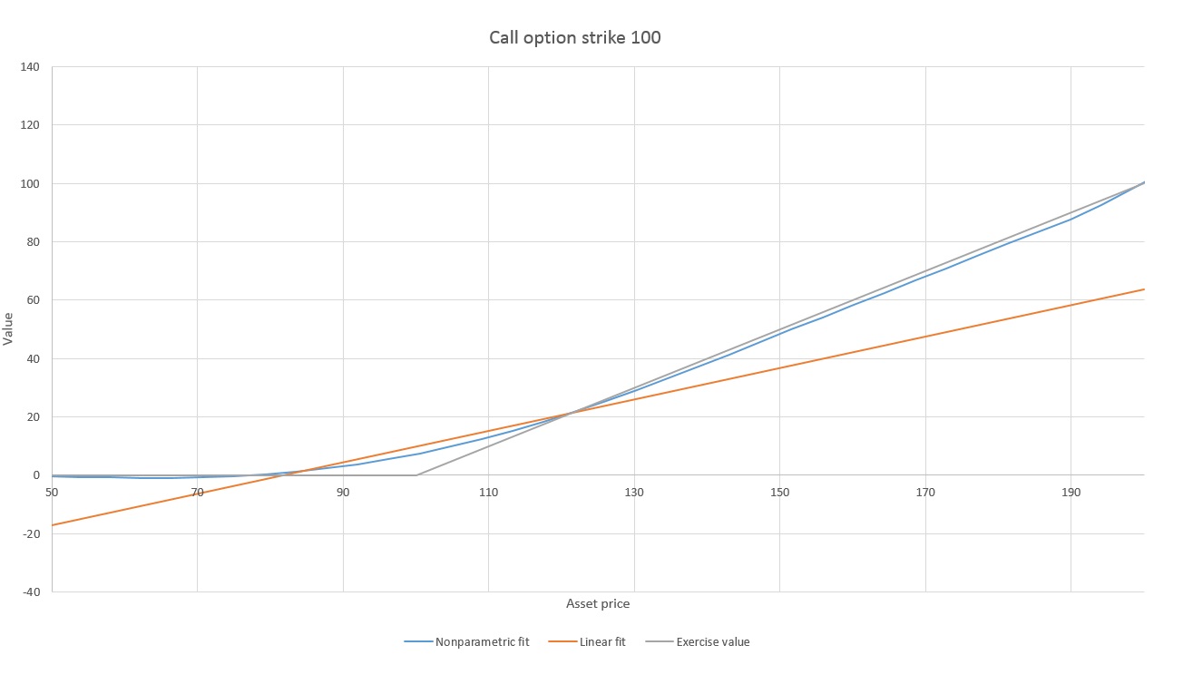
Actually, we first did a linear regression to come up with a rough initial approximation to use as a rough initial point for the optimization procedure. But this line has been fitted by optimization, not by regression. Note that the optimization procedure has succeeded in finding the exact crossover point at 122 of the much more sophisticated non-parametric fitting. And although a poor fit for the data, the linear fit is above and below the exercise value in exactly the right regions, so it makes exercise decisions perfectly.
So it seems like we can dispense with function fitting! The only piece of information we need are the places where the value of continuing “crosses over” the value of exercising (combined with knowing whether it is above or below in at least one region)
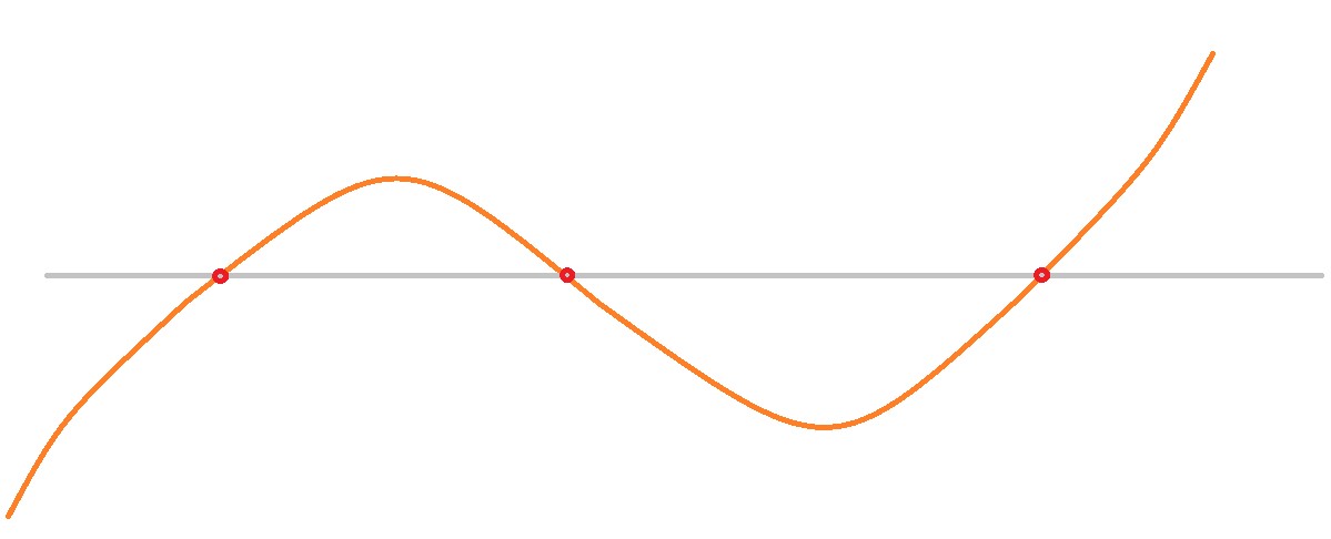
It’s clear that our optimization procedure will work splendidly whenever there is only one crossover point. What is there are many crossover points? One option is to use an optimization procedure to find a higher order polynomial to serve as our decision surface, as in the below illustration. We would need a polynomial of order equal to the number of crossovers.
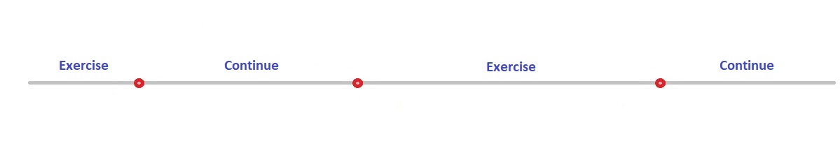
But do we need to bother with a function at all? It does offer one advantage – the ability to use a polynomial regression to generate a rough initial point for the optimization procedure. But the astute reader will notice that what we are looking at here is really a classification problem, not a function fitting problem at all. The information we are really trying to extract is the following:
 In the higher dimensional case where there is more than one underlying, the cross-over points are not points, but hypersurfaces. In the case of two underlyings for example, the cross-over boundary consists of one or more curves in the plane. Let’s consider what this would look like in the two dimensional case where there are two underlying assets to the derivative:

Here, each red “x” represents a data point where the value of exercising is greater than the value of continuing. Each blue “o” represents a data point where the reverse is true. Our task is to come up with the decision boundary which most accurately “classifies” the points into exercise vs continue. But this is looking exactly like a classification problem from machine learning! In particular, this problem is looking exactly like the sort of problem one can solve using a support vector machine (SVM)!
For the moment, we’ll leave this exploration there. Hopefully the reader has become convinced that there are some exciting possibilities for applying machine learning and optimization methods to the pricing of derivatives using the Longstaff-Schwartz method. Except, since we have dispensed with function fitting entirely, I’m not sure we can call this the Longstaff-Schwartz method anymore! Whatever it’s called, it’s an intriguing new approach to pricing derivatives with early exercise using Monte-Carlo. It would be interesting to conduct a study of these new methods and how they compare to a more conventional Longstaff-Schwartz approach.
Interested in developing code to price derivatives with early exercise? We offer derivative pricing consulting services, and a wide range of general quantitative analysis consulting services.