Genius Mathematics Consultants

Network reliability optimization problems first appeared for telecommunication and transport systems. These days, they also have applications in computer networks, and electric and gas networks. In the modern world, the consequences of a network failing can be catastrophic in terms of cost and even lives lost. Since many non-mathematical professionals need to design networks of various kinds, network optimization is a great example of how math consulting can deliver value for industry.

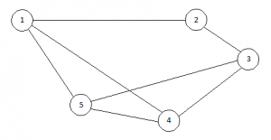
The goal of reliability optimization is to minimize the cost of the network, while ensuring it still meets some minimum standard of “reliability”, represented by the probability of the network failing.  Conceptually, a network can be represented by an undirected graph \(G = (N,E)\) with nodes \(N\) and edges \(E\):

Let \(x_{ij}\) represent which nodes we build connections between, i.e.\(x_{ij}=1\) if there is an edge between node \(i\) and node \(j\) and \(x_{ij}=0\) otherwise. Let \(c_{ij}\) represent the cost of building a connection between node \(i\) and node \(j\). Then the cost of building the network is

\[C(x) = \sum_{i=1}^{n-1} \sum_{j=i+1}^{n}c_{ij}x_{ij}.\]

Let \(p\) represent the probability that a node will be operational. There are two commonly used standards for when a network is considered to be operational, depending on the application:

1. Two specified nodes are connected
2. Every node is connected to every other node

It is then possible to assign to every network \(x\) a reliability \(R(x)\), which is the probability that the network will be operational. Suppose our tolerance for network failure is \(R_{min}\). Then we wish to minimize the cost function \(C(x)\) subject to the constraint \(R(x) \geq R_{min}\).

Mathematically speaking, network reliability problems are examples of integer programming problems, and can be solved in a variety of ways, such as using genetic algorithms.

A common choice of distribution for operational risk modelling is lognormal. This distribution has a fairly heavy tail and is mathematically and conceptually simple. Often a separate lognormal will be used to model the body and the tail of each risk cell, so that they can be parameterised separately. The body distribution can be chosen to closely match the common losses that occur in the internal data for that risk cell, which the tail can chosen to match the expectation of extreme losses. The necessity of this is questionable, since the high quantiles computed in op risk modelling are overwhelmingly driven by the tail. In most cases, if model simplicity is desired, a single distribution using the tail parameters is sufficient.

Once the loss severity distribution has been estimated for each risk cell, along with a corresponding frequency distribution (typically Poisson, although op risk models are not sensitive to this choice), then Monte Carlo simulation is used to sum them and produce the bank’s total or aggregate loss distribution. The modeller may then be surprised to discover that the median aggregate loss is far higher than the bank’s typical annual loss! After all, the median loss from the body distribution matches that in the internal data for each risk cell, so shouldn’t the  same be true of the aggregate distribution?

The explanation here lies in the heavy tailed nature of the lognormal distribution. In particular, the lognormal has the property that for large \(N\), the sum of \(N\) randomly generated losses approaches the maximum loss, i.e.

\[\sum_{i=1}^N x_i \to \max(\{x_i\}).\]

This means that, surprisingly, even a typical loss in the aggregate distribution (say, the median) is primarily constituted by a small number of tail losses from the individual distributions, and not losses near the medians! Thus, the medians of the individual distributions end up being pretty much irrelevant.

Of course, op risk models are typically constructed to estimate the 99.9% quantile, not the median (which banks have data for anyway). However, it is instructive to note that it is very difficult to model op risk in a way that accurately reproduces both the extreme losses, and the more common losses, due to the heavy tailed nature of the distributions.

This illustration shows how even relatively simple financial modelling problems can result in technical complexities that are very difficult for finance profressionals to understand and resolve. This is a great example of how our quantitative analysis consulting services can deliver great value and impress the regulators!

Anyone who has worked in financial risk modelling can testify to the fact that Monte Carlo simulations can take a long time to run – sometimes an entire day or longer! The problem this causes is that model testing – particularly sensitivity testing around the inputs, parameters and methodologies – ends up taking weeks and months. The loss in productivity (and the sanity of the modeler) is huge.

This is a really simple technique that can reduce run time by as much as half.

Often, risk modelers are interested in simulating from an aggregate distribution that is the sum of multiple other distributions. Usually it is the very high quantiles of this aggregate distribution that they want to estimate, such as the 99.9% quantile or 1 in 1000 event.  They would therefore like to generate a lot of losses from the tail of the distribution, to get sufficient resolution for estimating the high quantiles. Unfortunately, by definition most of the losses generated during a Monte Carlo simulation will not fall in the tail of the constituent distributions, and 50% will even fall below the median. for heavy-tailed distributions, these small losses usually don’t contribute much to the large losses in the aggregate distribution. This means that a tremendous amount of computational power is used to generate high density losses in the body of the distribution, just to get a handful of losses in the tail.

The solution: re-use those body losses! Put a cap on the number of body losses you wish to generate, say 10,000 losses below the 90% quantile. Before beginning the Monte Carlo simulation, generate these 10,000 losses and store them in a vector. Now, whenever the simulation calls for a loss below the 90% quantile, simply locate the nearest corresponding loss in this vector. In other words, if the random number generates the number 0.44, we would calculate 0.44*10,000 and round to the nearest whole number and use the loss with the corresponding index. This procedure is much faster than the calculations required to invert a lognormal cdf. However, losses above the 90% quantile should continue to be uniquely generated to preserve accuracy in the tail.

While there are more sophisticated approaches to improving Monte Carlo performance, a simple approach like this is quick to implement and less prone to errors.

Another tip that’s handy to know is that with certain distributions, there may be a shortcut that doesn’t require you to generate all the losses again when you change a parameter. For a lognormal distribution, for example, the losses generated are proportional to \(\exp(\mu)\). This means that if wish to change the \(\mu\) parameter from \(\mu_1\) to \(\mu_2\), all you have to do is scale all the losses by \(\exp(\mu_2-\mu_1)\)! This can save a tremendous amount of time when conducting sensitivity testing.

Does your bank have Monte Carlo models which take all day to run? Why not drop us an email to find out how our financial modelling consulting services can work for you.