Genius Mathematics Consultants

As our world becomes more complex, fields of expertise are becoming more and more specialised. As knowledge grows, the amount any one person can be an expert in gets smaller. This means that now, more than ever, collaboration is the name of the game. You might like to take a look at Sciencemag’s article on successful collaboration, or the European Science Foundation’s publication on mathematics in industry.

There are no shortage of success stories demonstrating the applicability of mathematics to science and industry. As one of the most fundamental and abstract subjects, mathematics may be without peer in the broadness of its applications. Perhaps for no other discipline is it so important to form lines of communication and collaboration with other experts. And as the world becomes increasingly technically sophisticated, this fact will become ever more true. It’s important for both sides to determine a strategy through which mathematicians and other experts can strengthen their interactions to prepare for our highly technological future.

It sometimes doesn’t occur to people that their industry should seek the the expertise of mathematicians. Sometimes, this is because mathematics in their industry is working its magic under a different name or job title, such as engineer. They may not even be aware that there is such a thing as a math consultant, and therefore unlikely to seek one out. The completion of a PhD in a field of mathematics not only qualifies the holder within that field, but testifies to an ability to think creatively and solve difficult problems. Ironically, these skills make mathematicians the ideal consultants – even for problems that are not explicitly mathematical. They lend themselves so well to applied research and development tasks that the concept of a math consulting firm should be part of the lingo.

Encouragingly, surveys have found that managers express enthusiasm for collaborating with mathematicians, and genuinely believe that mathematics can provide them with a competitive edge. Yet, their own lack of familiarity with mathematics can make it difficult for them to drive the interaction from their side, and to generate project ideas.

So how can math consultants and other professionals improve collaboration?

• Both sides should work to build professional connections with each other, even before any possible collaborative projects are apparent to either side. These connections may yield unforeseen fruit in the future.
• Scientists, engineers and other professionals should discuss with mathematicians problems they are working on or facing in their fields. After all, you never know what value they may be able to add if they were only aware of the problem!
• Since other professionals may not know enough about what mathematicians do to realise when they are needed, math consultants may need to “take it to them”. Mathematicians need to invest time in learning about the work being done in science and industry, and develop their own project proposals to present to industry leaders.
• Many businesses and teams do not include a mathematician who would have the skills to solve difficult quantitative problems that arise in their field. Historically, this made it difficult for collaboration to occur. And increasing specialisation means teams would get larger and larger if they needed a permanent team member for every area of expertise that arises. Fortunately, the internet has created an unprecedented flexibility for working which means that you needn’t employ a full-time mathematician to reap the benefits. The expertise you need is only a few clicks away. Industry professionals should embrace online consulting as a convenient and cost-effective way to tap into the expertise of mathematicians

\(\)You might assume that one of the largest financial consulting firms in the world with a net revenue in the tens of billions would be able to do some pretty good capital and risk modelling work. As a mathematician working in finance, I’ve come to realise that even the largest and most prestigious financial organisations routinely make critical errors in the design and validation of financial models. This is true not just for complex models, but even very simple ones.

In this article we’ll take a look at some risk modelling work performed by one of the “big four” financial consulting firms. The model is supposed to estimate how much capital a bank should hold to protect itself against large losses. As we’ll see, they could have hired Chim-Chim the monkey to design and validate a risk model for them with similar results (but at a significant cost advantage!)

So here’s what they did. A business manager, let’s call him “Bob”, used his knowledge of the business and memory of past losses to estimate the loss size that could occur in each part of the business, and on average how many years would pass before such a loss occurred. They divided each loss size by the corresponding numbers of years to yield a set of data points, to which they fitted a lognormal distribution by matching mean and variance, as given by the following formulae:

\[mu = \log(m^2 / \sqrt{v + m^2}),\]

\[\sigma = \sqrt{log(v/m^2 + 1}).\]

The bank determined that it would hold as capital the 99.9% quantile of the resulting distribution.

Let’s say bob comes up with loss estimates of $50 million every 5 years, $30 million every 3 years, and $25 million every 2 years. If you determine the parameters of the lognormal distribution from the above formulae and find the 99.9% quantile, you’ll get $16.2 million. The model provided by the financial consulting firm predicts that the bank should hold $16.2 million in capital, which will allegedly protect it against all but the 1 in a thousand year loss.

So what’s wrong with this approach?

First, think about the numbers – if we suffer a loss of $50 million every 5 years, how can $16.2 million cover the once in a thousand year loss! It doesn’t even cover the once in 5 year loss from only one of the three parts of the business! Clearly there’s something very wrong with this modelling work!

Next, let’s see if the model output changes in a reasonable way when we make a change to the input. Suppose Bob realises that he has forgotten about one important risk. You see, bob occasionally loses his pen. He estimates that he loses his pen about once a year, and that it costs the bank about $1 to replace it. Our consulting firm adds this data point to the model inputs and redoes the calculation. So what is the result now? Has the amount of capital gone up by a few bucks? Nope, it’s now $45.3 million! In order to insure bob against the risk of losing his pen, the bank has to hold an additional $29.2 million in capital! In fact, the cost of insuring that pen is almost twice as much as the $16.2 million required to ensure the entire business!

Ok, so this model is crazy. But what’s wrong from a mathematical perspective?

These analysts know about fitting a lognormal distribution to data, but there’s no depth to their understanding, causing them to design models that produce entirely meaningless numbers. When you fit a lognormal distribution to some data, you are making the assumption that the data is lognormally distributed. The data you are using therefore has to be representative of amounts chosen at random from the loss distribution. Because the standard deviation of the distribution is fixed to the standard deviation of the estimates, the closer together the estimates are, the smaller the amount of capital the model estimates!

But the data they were using was a fairly arbitrary collection of numbers gathered by considering different loss scenarios in different parts of the business. How spread out these numbers were was not something they were even conscious of – yet it was the critical determinant of risk. If Bob comes up with a few losses close together, the model won’t require the bank to hold much capital – even if those losses are very large. But if Bob comes up with losses far apart – even much smaller ones – then the model will require the bank to hold a huge amount of capital!

You would think banks would be outraged that they were paying so much money for models that were nothing but random number generators, and concerned that they weren’t holding the right amount of capital to prevent their business from collapsing. And it’s certainly not very good for the security of their customer’s money. How much money do you this financial consulting firm, one of the top four, charged for Chim-Chim the monkey numbers? If only the CEO knew how much money he paid external consultants to pretend to do risk modelling.

Can you believe these large financial consulting firms get paid a lot of money to validate risk models?

So, if you’re seeking professional financial modelling consulting, you could hire me to produce quality, meaningful capital numbers that will protect your business against unexpected losses. Or you could hire one of the big four to take a random stab in the dark while tripping over the washing basket – for ten times the cost!

Interested in applying machine learning to your business, but not sure where to start?

Having heard about the many spectacular achievements of machine learning and it’s growing adoption, many businesses are keen to use it to gain competitive advantage. And, worried about being left behind if they don’t!

However, despite grand ambitions, the rapid growth of the field means there is a lack of people with the expertise to implement actual working solutions. Many businesses are in the position of having a lot of data, but no idea how they can use it!

Machine learning has been applied to such a diverse set of applications that one can only sample them:

• Predicting which units are faulty early in a production line rather than late, to reduce wastage
• Automatic fruit grading, sorting and shelf-life estimation based on attributes like weight, shape, and colour
• Predicting which machine parts are likely to fail and when, to optimize when machine parts are replaced or scheduled for maintenance. A solution must be found which optimizes how limited maintenance and replacement budget is spent, while also minimizing failure and lost profit due to downtime
• Optimizing the structure of a network to minimize the probability of failure for a given network cost
• Automation of human roles in industry and manufacturing
• Optimizing system configurations based on input like weather data, time of year, order numbers etc.

We’re interested in developing mutually beneficial collaborations with industry. To that end, we’d be interested in helping you explore if and how machine learning can increase profits, reduce wastage, and optimize the efficiency of your business.

Please explore the site to learn more about our algorithm consulting services (we offer general math consulting as well). Then, we’d love to get this conversation started, so please contact us to express your interest!

Remote sensing systems (such as LIDAR) allow us to measure a plethora of variables on the earth’s surface and in the air. This includes temperature, wind, vegetation, clouds, ice and many more. However, the relationship between the variable to be measured and the signal received can be complex, as radiation passing through the atmosphere is scattered and absorbed by clouds and molecules in the atmosphere. Attempting to determine this relationship using theory alone may be arduous. Machine learning is a natural alternative.

Let \(v\) denote some variable we wish to measure (perhaps on the earth’s surface), and \(s\) the signal received by the sensor (possibly located on a satellite). We wish to find a relationship

\[v = f(s),\]

that will allow us to convert the properties of the signal, which may contain data from several frequency bands, to the properties we actually wish to measure. Suppose we have gathered a large number of data pairs \((s_i,v_i)\). We can do this be recording the signal received \(s_i\) when the sensor is pointed at a location whose properties \(v_i\) are already known. We then use these data points to train or teach a neural network.

Ideally, the data used for fitting is only a subset of the total amount of data collected, so that the neural network can be cross-validated against data that was not used in the fitting process.

Machine learning has been applied to remote sensing in many practical applications including:

• Measuring the chlorophyll concentration in the ocean
• Classifying vegetation
• Classifying cloud types
• Measuring precipitation
• Identifying snow cover
• Forecasting

Of course, remote sensing is only one of an unlimited number of applications of machine learning. Whenever you wish to determine a relationship present in your data that may be too complex to determine using scientific theory, machine learning is an exciting alternative.

Network reliability optimization problems first appeared for telecommunication and transport systems. These days, they also have applications in computer networks, and electric and gas networks. In the modern world, the consequences of a network failing can be catastrophic in terms of cost and even lives lost. Since many non-mathematical professionals need to design networks of various kinds, network optimization is a great example of how math consulting can deliver value for industry.

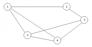
The goal of reliability optimization is to minimize the cost of the network, while ensuring it still meets some minimum standard of “reliability”, represented by the probability of the network failing.  Conceptually, a network can be represented by an undirected graph \(G = (N,E)\) with nodes \(N\) and edges \(E\):

Let \(x_{ij}\) represent which nodes we build connections between, i.e.\(x_{ij}=1\) if there is an edge between node \(i\) and node \(j\) and \(x_{ij}=0\) otherwise. Let \(c_{ij}\) represent the cost of building a connection between node \(i\) and node \(j\). Then the cost of building the network is

\[C(x) = \sum_{i=1}^{n-1} \sum_{j=i+1}^{n}c_{ij}x_{ij}.\]

Let \(p\) represent the probability that a node will be operational. There are two commonly used standards for when a network is considered to be operational, depending on the application:

1. Two specified nodes are connected
2. Every node is connected to every other node

It is then possible to assign to every network \(x\) a reliability \(R(x)\), which is the probability that the network will be operational. Suppose our tolerance for network failure is \(R_{min}\). Then we wish to minimize the cost function \(C(x)\) subject to the constraint \(R(x) \geq R_{min}\).

Mathematically speaking, network reliability problems are examples of integer programming problems, and can be solved in a variety of ways, such as using genetic algorithms.

A common choice of distribution for operational risk modelling is lognormal. This distribution has a fairly heavy tail and is mathematically and conceptually simple. Often a separate lognormal will be used to model the body and the tail of each risk cell, so that they can be parameterised separately. The body distribution can be chosen to closely match the common losses that occur in the internal data for that risk cell, which the tail can chosen to match the expectation of extreme losses. The necessity of this is questionable, since the high quantiles computed in op risk modelling are overwhelmingly driven by the tail. In most cases, if model simplicity is desired, a single distribution using the tail parameters is sufficient.

Once the loss severity distribution has been estimated for each risk cell, along with a corresponding frequency distribution (typically Poisson, although op risk models are not sensitive to this choice), then Monte Carlo simulation is used to sum them and produce the bank’s total or aggregate loss distribution. The modeller may then be surprised to discover that the median aggregate loss is far higher than the bank’s typical annual loss! After all, the median loss from the body distribution matches that in the internal data for each risk cell, so shouldn’t the  same be true of the aggregate distribution?

The explanation here lies in the heavy tailed nature of the lognormal distribution. In particular, the lognormal has the property that for large \(N\), the sum of \(N\) randomly generated losses approaches the maximum loss, i.e.

\[\sum_{i=1}^N x_i \to \max(\{x_i\}).\]

This means that, surprisingly, even a typical loss in the aggregate distribution (say, the median) is primarily constituted by a small number of tail losses from the individual distributions, and not losses near the medians! Thus, the medians of the individual distributions end up being pretty much irrelevant.

Of course, op risk models are typically constructed to estimate the 99.9% quantile, not the median (which banks have data for anyway). However, it is instructive to note that it is very difficult to model op risk in a way that accurately reproduces both the extreme losses, and the more common losses, due to the heavy tailed nature of the distributions.

This illustration shows how even relatively simple financial modelling problems can result in technical complexities that are very difficult for finance profressionals to understand and resolve. This is a great example of how our quantitative analysis consulting services can deliver great value and impress the regulators!

Anyone who has worked in financial risk modelling can testify to the fact that Monte Carlo simulations can take a long time to run – sometimes an entire day or longer! The problem this causes is that model testing – particularly sensitivity testing around the inputs, parameters and methodologies – ends up taking weeks and months. The loss in productivity (and the sanity of the modeler) is huge.

This is a really simple technique that can reduce run time by as much as half.

Often, risk modelers are interested in simulating from an aggregate distribution that is the sum of multiple other distributions. Usually it is the very high quantiles of this aggregate distribution that they want to estimate, such as the 99.9% quantile or 1 in 1000 event.  They would therefore like to generate a lot of losses from the tail of the distribution, to get sufficient resolution for estimating the high quantiles. Unfortunately, by definition most of the losses generated during a Monte Carlo simulation will not fall in the tail of the constituent distributions, and 50% will even fall below the median. for heavy-tailed distributions, these small losses usually don’t contribute much to the large losses in the aggregate distribution. This means that a tremendous amount of computational power is used to generate high density losses in the body of the distribution, just to get a handful of losses in the tail.

The solution: re-use those body losses! Put a cap on the number of body losses you wish to generate, say 10,000 losses below the 90% quantile. Before beginning the Monte Carlo simulation, generate these 10,000 losses and store them in a vector. Now, whenever the simulation calls for a loss below the 90% quantile, simply locate the nearest corresponding loss in this vector. In other words, if the random number generates the number 0.44, we would calculate 0.44*10,000 and round to the nearest whole number and use the loss with the corresponding index. This procedure is much faster than the calculations required to invert a lognormal cdf. However, losses above the 90% quantile should continue to be uniquely generated to preserve accuracy in the tail.

While there are more sophisticated approaches to improving Monte Carlo performance, a simple approach like this is quick to implement and less prone to errors.

Another tip that’s handy to know is that with certain distributions, there may be a shortcut that doesn’t require you to generate all the losses again when you change a parameter. For a lognormal distribution, for example, the losses generated are proportional to \(\exp(\mu)\). This means that if wish to change the \(\mu\) parameter from \(\mu_1\) to \(\mu_2\), all you have to do is scale all the losses by \(\exp(\mu_2-\mu_1)\)! This can save a tremendous amount of time when conducting sensitivity testing.

Does your bank have Monte Carlo models which take all day to run? Why not drop us an email to find out how our financial modelling consulting services can work for you.